(Deep) Kernel Mean Embeddings
for Representing and Learning on Distributions
Danica J. Sutherland(she/her)
University of British Columbia + Amii
Lifting Inference with Kernel Embeddings (LIKE-23), June 2023
This talk: how to lift inference with kernel embeddings
Slides at djsutherland.ml/slides/like23
(Swipe or arrow keys to move through slides; for a menu to jump; for more.)
PDF version at djsutherland.ml/slides/like23.pdf
HTML version at djsutherland.ml/slides/like23
Part I: Kernels
Why kernels?
- Machine learning! …but how do we actually do it?
- Linear models! ,
- Extend …
- Kernels are basically a way to study doing this
with any, potentially very complicated, - Convenient way to make models on documents, graphs, videos, datasets, probability distributions, …
- will live in a reproducing kernel Hilbert space
Hilbert spaces
- A complete (real or complex) inner product space
- Inner product space: a vector space with an inner product:
- for ,
- Complete: “well-behaved” (Cauchy sequences have limits in )
Kernel: an inner product between feature maps
- Call our domain , some set
- , functions, distributions of graphs of images, …
- is a kernel on if there exists a Hilbert space and a feature map so that
- Roughly, is a notion of “similarity” between inputs
- Linear kernel on :
Aside: the name “kernel”
- Our concept: "positive semi-definite kernel," "Mercer kernel," "RKHS kernel"
- Exactly the same: GP covariance function
- Semi-related: kernel density estimation
- , usually symmetric, like RKHS kernel
- Always requires , unlike RKHS kernel
- Often requires , unlike RKHS kernel
- Not required to be inner product, unlike RKHS kernel
- Unrelated:
- The kernel (null space) of a linear map
- The kernel of a probability density
- The kernel of a convolution
- CUDA kernels
- The Linux kernel
- Popcorn kernels
Building kernels from other kernels
- Scaling: if , is a kernel
- Sum: is a kernel
- Is necessarily a kernel?
- Take , , .
- Then
- But .
Positive definiteness
- A symmetric function
i.e.
is positive semi-definite
if for all , , , - Equivalent: kernel matrix is psd (eigenvalues )
- Hilbert space kernels are psd
- psd functions are Hilbert space kernels
- Moore-Aronszajn Theorem; we'll come back to this
Some more ways to build kernels
- Limits: if exists, is psd
- Products: is psd
- Let , be independent
- Covariance matrices are psd, so is too
- Powers: is pd for any integer
, the polynomial kernel
- Exponents: is pd
- If , is pd
- Use the feature map
, the Gaussian kernel
Reproducing property
- Recall original motivating example with
- Kernel is
- Classifier based on linear
- is the function itself; corresponds to vector in
is the function evaluated at a point - Elements of are functions,
- Reproducing property: for
Reproducing kernel Hilbert space (RKHS)
- Every psd kernel on defines a (unique) Hilbert space, its RKHS ,
and a map where- Elements are functions on , with
- Combining the two, we sometimes write
- is the evaluation functional
An RKHS is defined by it being continuous, or
Moore-Aronszajn Theorem
- Building for a given psd :
- Start with
- Define from
- Take to be completion of in the metric from
- Get that the reproducing property holds for in
- Can also show uniqueness
- Theorem: is psd iff it's the reproducing kernel of an RKHS
A quick check: linear kernels
- on
- “corresponds to”
- If , then
- Closure doesn't add anything here, since is closed
- So, linear kernel gives you RKHS of linear functions
More complicated: Gaussian kernels
- is infinite-dimensional
- Functions in are bounded:
- Choice of controls how fast functions can vary:
- Can say lots more with Fourier properties
Kernel ridge regression
Linear kernel gives normal ridge regression: Nonlinear kernels will give nonlinear regression!
How to find ? Representer Theorem:
- Let , and its orthogonal complement in
- Decompose with ,
- Minimizer needs , and so
Setting derivative to zero gives
satisfied by
Kernel ridge regression and GP regression
- Compare to regression with prior, observation noise
- If we take , KRR is exactly the GP regression posterior mean
- Note that GP posterior samples are not in , but are in a slightly bigger RKHS
- Also a connection between posterior variance and KRR worst-case error
- For many more details:
![]()
Other kernel algorithms
- Representer theorem applies if is strictly increasing in
- Kernel methods can then train based on kernel matrix
- Classification algorithms:
- Support vector machines: is hinge loss
- Kernel logistic regression: is logistic loss
- Principal component analysis, canonical correlation analysis
- Many, many more…
- But not everything works...e.g. Lasso regularizer
Some very very quick theory
- Generalization: how close is my training set error to the population error?
- Say , consider , -Lipschitz loss
- Rademacher argument implies expected overfitting
- If “truth” has low RKHS norm, can learn efficiently
- Approximation: how big is RKHS norm of target function?
- For universal kernels, can approximate any target with finite norm
- Gaussian is universal 💪 (nothing finite-dimensional can be)
- But “finite” can be really really really big
Limitations of kernel-based learning
- Generally bad at learning sparsity
- e.g. for large
- Provably statistically slower than deep learning for a few problems
- e.g. to learn a single ReLU, , need norm exponential in [Yehudai/Shamir NeurIPS-19]
- Also some hierarchical problems, etc [Kamath+ COLT-20]
- Generally apply to learning with any fixed kernel
- computational complexity, memory
- Various approximations you can make
Part II: (Deep) Kernel Mean Embeddings
Mean embeddings of distributions
- Represent point as :
- Represent distribution as :
- Last step assumed (Bochner integrability)
- Okay. Why?
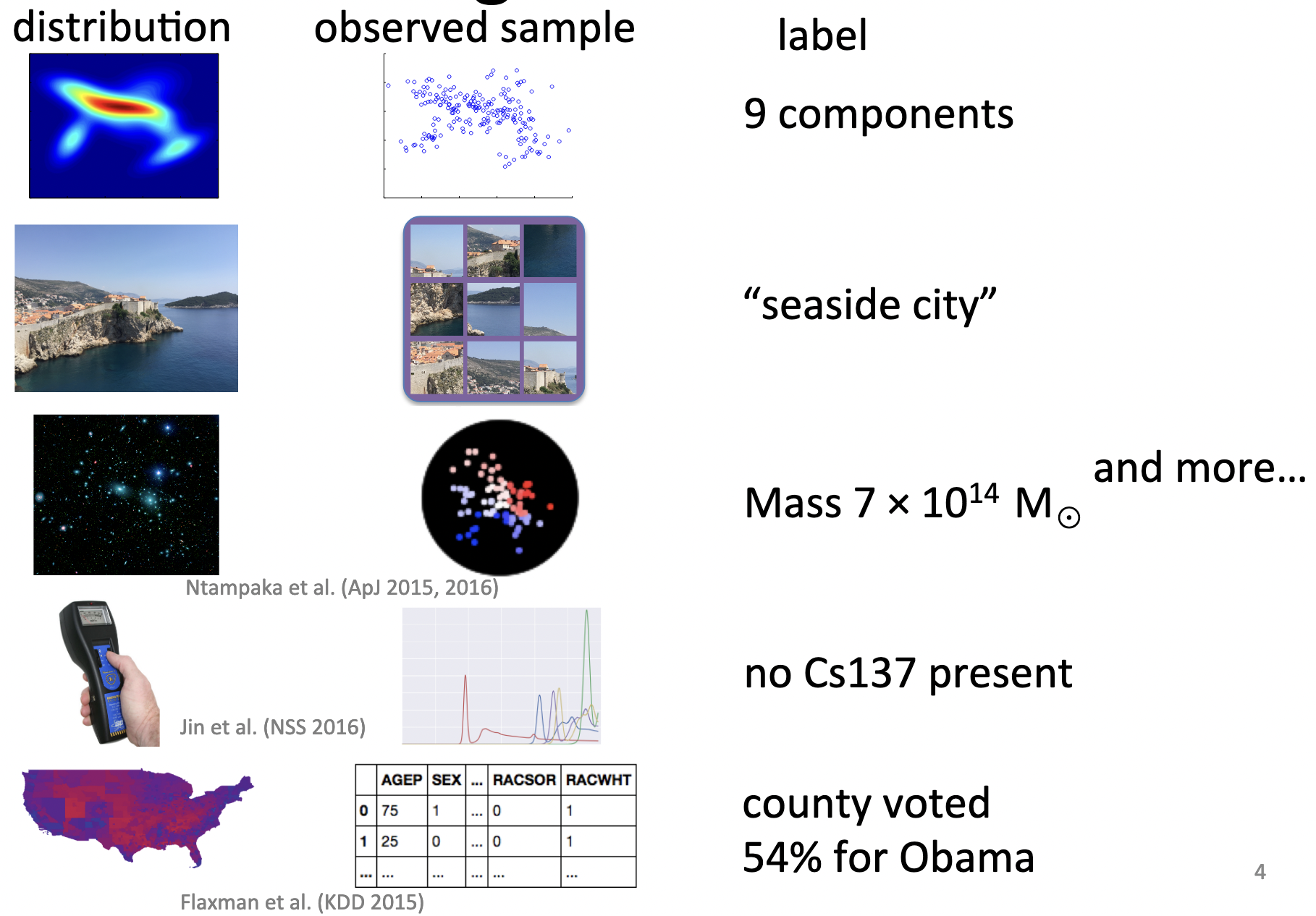
- One reason: ML on distributions [Szabó+ JMLR-16]
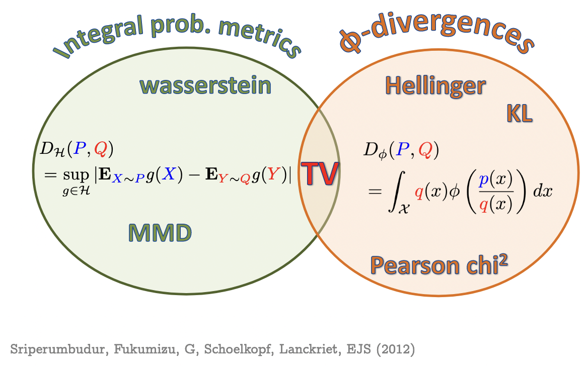
- More common reason: comparing distributions
Maximum Mean Discrepancy
- Last line is Integral Probability Metric (IPM) form
- is called “witness function” or “critic”: high on , low on
MMD properties
- , symmetry, triangle inequality
- If is characteristic, then iff
- i.e. is injective
- Makes MMD a metric on probability distributions
- Universal characteristic
- If we use a linear kernel:
- just Euclidean distance between means
- If we use ,
the squared MMD becomes the energy distance [Sejdinovic+ Annals-13]
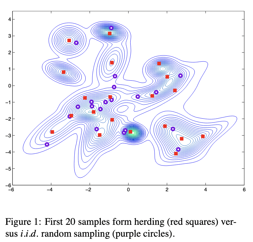
Application: Kernel Herding
- Want a "super-sample" from : for all
- Letting , want for all
- Error
- Greedily minimize the MMD:
- Get approximation instead of with random samples
Estimating MMD from samples
 |  |  | |
|---|---|---|---|
| 1.0 | 0.2 | 0.6 |
| 0.2 | 1.0 | 0.5 |
| 0.6 | 0.5 | 1.0 |
 |  | ||
|---|---|---|---|
| 1.0 | 0.8 | 0.7 | |
| 0.8 | 1.0 | 0.6 |
| 0.7 | 0.6 | 1.0 |
| | | |
|---|---|---|---|
| 0.3 | 0.1 | 0.2 | |
| 0.2 | 0.3 | 0.3 |
| 0.2 | 0.1 | 0.4 |
MMD vs other distances
- MMD has easy estimator
- block or incomplete estimators are for , but noisier
- For bounded kernel, estimation error
- Independent of data dimension!
- But, no free lunch…the value of the MMD generally shrinks with growing dimension, so constant error gets worse relatively
GP view of MMD
- Optimizing the gap in average-case gap sampled from GP
- Six-line proof [Kanagawa+ 18, Proposition 6.1]
Application: Two-sample testing
- Given samples from two unknown distributions
- Question: is ?
- Hypothesis testing approach:
- Reject if
- Do smokers/non-smokers get different cancers?
- Do Brits have the same friend network types as Americans?
- When does my laser agree with the one on Mars?
- Are storms in the 2000s different from storms in the 1800s?
- Does presence of this protein affect DNA binding? [MMDiff2]
- Do these dob and birthday columns mean the same thing?
- Does my generative model match ?
What's a hypothesis test again?
MMD-based testing
- : converges in distribution to…something
- Infinite mixture of s, params depend on and
- Can estimate threshold with permutation testing
- : asymptotically normal
- Any characteristic kernel gives consistent test…eventually
- Need enormous if kernel is bad for problem
Classifier two-sample tests

- is the accuracy of on the test set
- Under , classification impossible:
- With where ,
get
Deep learning and deep kernels
- is one form of deep kernel
- Deep models are usually of the form
- With a learned
- If we fix , have with
- Same idea as NNGP approximation
- Generalize to a deep kernel:
Normal deep learning deep kernels
- Take
- Final function in will be
- With logistic loss: this is Platt scaling
“Normal deep learning deep kernels” – so?
- This does not say that deep learning is (even approximately) a kernel method
- …despite what some people might want you to think
![]()
- We know theoretically deep learning can learn some things faster than any kernel method [see Malach+ ICML-21 + refs]
- But deep kernel learning ≠ traditional kernel models
- exactly like how usual deep learning ≠ linear models

Optimizing power of MMD tests
- Asymptotics of give us immediately that , , are constants: first term usually dominates
- Pick to maximize an estimate of
- Use from before, get from U-statistic theory
- Can show uniform convergence of estimator
- Get better tests (even after data splitting)
Application: (S)MMD GANs
- An implicit generative model:
- A generator net outputs samples from
- Minimize estimate of on a minibatch
- MMD GAN:
- SMMD GAN:
- Scaled MMD uses kernel properties to ensure smooth loss for
by making witness function smooth [Arbel+ NeurIPS-18] - Uses
- Standard WGAN-GP better thought of in kernel framework
- Scaled MMD uses kernel properties to ensure smooth loss for
Application: fair representation learning (MMD-B-FAIR) [Deka/Sutherland AISTATS-23]
- Want to find a representation where
- We can tell whether an applicant is “creditworthy”
- We
can't distinguish applicants by race
- Find a good classifier with near-zero test power for race
- Minimizing the test power criterion turns out to be hard
- Workaround: minimize test power of a (theoretical) block test
Application: distribution regression/classification/…
- We can define a kernel on distributions by, e.g.,
- Some pointers:
[Muandet+ NeurIPS-12] [Sutherland 2016] [Szabó+ JMLR-16]
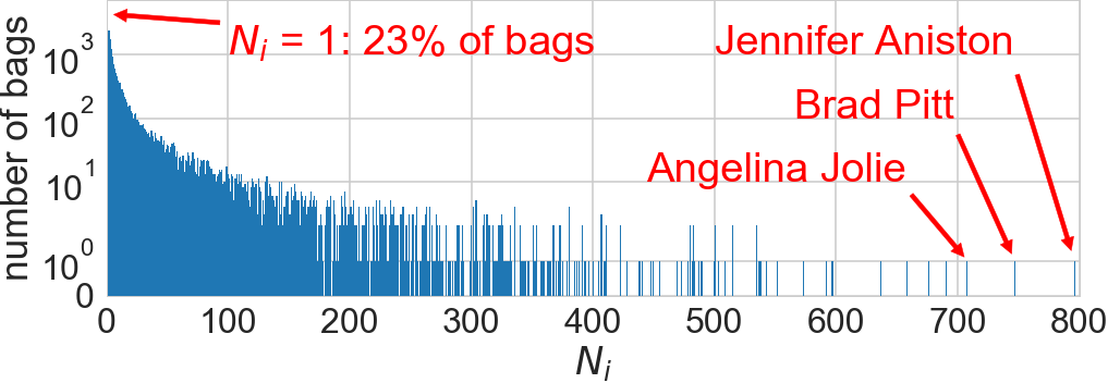
Example: age from face images [Law+ AISTATS-18]
Bayesian distribution regression: incorporate uncertainty
 ,
,  ,
,  ,
,  ,
, 
IMDb database [Rothe+ 2015]: 400k images of 20k celebrities

Independence
- iff for all square-integrable ,
- Let's implement for RKHS functions , :where is
Cross-covariance operator and independence
- If , then
- If ,
- If , are characteristic:
- implies [Szabó/Sriperumbudur JMLR-18]
- iff
- iff (sum squared singular values)
- HSIC: "Hilbert-Schmidt Independence Criterion"
HSIC
- Linear case: is cross-covariance matrix, HSIC is squared Frobenius norm
- Default estimator (biased, but simple): ,
HSIC applications
- Independence testing [Gretton+ NeurIPS-07]
- Clustering [Song+ ICML-07]
- Feature selection [Song+ JMLR-12]
- HSIC Bottleneck: alternative to backprop [Ma+ AAAI-20]
- biologically plausible(ish) [Pogodin+ NeurIPS-20]
- more robust [Wang+ NeurIPS-21]
- Self-supervised learning [Li+ NeurIPS-21]
- maybe better explanation of why InfoNCE/etc work
- ⋮
- Broadly: easier-to-estimate, sometimes-nicer version of mutual information
Example: SSL-HSIC [Li+ NeurIPS-21]
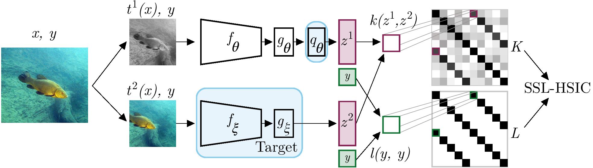
- Maximizes dependence between image features and its identity on a minibatch
- Using a learned deep kernel based on
Recap
- Point embedding : if then
- Mean embedding : if then
- is 0 iff (for characteristic kernels)
- is 0 iff
(for characteristic , ...or slightly weaker) - Often need to learn a kernel for good performance on complicated data
- Can often do end-to-end for downstream loss, asymptotic test power, …
More resources
- Berlinet and Thomas-Agnan, RKHS in Probability and Statistics
- kernels in general + mean embedding basics
- Steinwart and Christmann, Support Vector Machines
- kernels in general, learning theory
- Course slides by Julien Mairal + Jean-Philippe Vert
- kernels in general, learning theory
- Course materials by Arthur Gretton
- kernels in general, mean embeddings, MMD/HSIC
- Connections to Gaussian processes [Kanagawa+ 'GPs and Kernel Methods' 2018]
- Mean embeddings: survey [Muandet+ 'Kernel Mean Embedding of Distributions']
- These slides are at djsutherland.ml/slides/like23