\definecolor{cb1}{RGB}{76,114,176}
\definecolor{cb2}{RGB}{221,132,82}
\definecolor{cb3}{RGB}{85,168,104}
\definecolor{cb4}{RGB}{196,78,82}
\definecolor{cb5}{RGB}{129,114,179}
\definecolor{cb6}{RGB}{147,120,96}
\definecolor{cb7}{RGB}{218,139,195}
\DeclareMathOperator*{\argmin}{arg\,min}
\DeclareMathOperator*{\argmax}{arg\,max}
\newcommand{\bigO}{\mathcal{O}}
\newcommand{\bigO}{\mathcal{O}}
\newcommand{\bSigma}{\mathbf{\Sigma}}
\newcommand{\D}{\mathcal{D}}
\DeclareMathOperator*{\E}{\mathbb{E}}
\newcommand{\eye}{\mathbf{I}}
\newcommand{\F}{\mathbf{F}}
\newcommand{\K}{\mathcal{K}}
\newcommand{\Lip}{\mathrm{Lip}}
\DeclareMathOperator{\loss}{\mathit{L}}
\DeclareMathOperator{\lossdist}{\loss_\D}
\DeclareMathOperator{\losssamp}{\loss_\samp}
\newcommand{\N}{\mathcal{N}}
\newcommand{\norm}[1]{\lVert #1 \rVert}
\newcommand{\Norm}[1]{\left\lVert #1 \right\rVert}
\newcommand{\op}{\mathit{op}}
\newcommand{\samp}{\mathbf{S}}
\newcommand{\R}{\mathbb{R}}
\newcommand{\tp}{^{\mathsf{T}}}
\DeclareMathOperator{\Tr}{Tr}
\newcommand{\w}{\mathbf{w}}
\newcommand{\wmn}{\hat{\w}_{\mathit{MN}}}
\newcommand{\wmr}{\hat{\w}_{\mathit{MR}}}
\newcommand{\x}{\mathbf{x}}
\newcommand{\X}{\mathbf{X}}
\newcommand{\Y}{\mathbf{y}}
\newcommand{\y}{\mathrm{y}}
\newcommand{\z}{\mathbf{z}}
\newcommand{\zero}{\mathbf{0}}
\newcommand{\Scol}[1]{{\color{cb1} #1}}
\newcommand{\Jcol}[1]{{\color{cb2} #1}}
\newcommand{\dS}{\Scol{d_S}}
\newcommand{\dJ}{\Jcol{d_J}}
\newcommand{\xS}{\Scol{\x_S}}
\newcommand{\xJ}{\Jcol{\x_J}}
\newcommand{\XS}{\Scol{\X_S}}
\newcommand{\XJ}{\Jcol{\X_J}}
\newcommand{\wS}{\Scol{\w_S}}
\newcommand{\wsS}{\Scol{\w_S^*}}
\newcommand{\wJ}{\Jcol{\w_J}}
\newcommand{\wlam}{\Scol{\hat{\w}_{\lambda_n}}}
Can Uniform Convergence Danica J. Sutherland (she/her) University of British Columbia (UBC) / Alberta Machine Intelligence Institute (Amii)
NYU Center for Data Science – November 10, 2021
(Swipe or arrow keys to move through slides;
m
?
The
HTML version
is the “official” version,
though this PDF is basically the same.
Supervised learning Given i.i.d. samples
\samp = \{(\x_i, y_i)\}_{i=1}^n \sim \D^n
features/covariates
\x_i \in \R^d
y_i \in \R
Want
f
f(\x) \approx y
\D
:
f^* = \argmin\left[ \lossdist(f) := \E_{(\x, \y) \sim \D} \loss(f(\x), \y) \right]
e.g. squared loss:
L(\hat y, y) = (\hat y - y)^2
Standard approaches based on empirical risk minimization:
\hat{f} \approx \argmin\left[ \losssamp(f) := \frac1n \sum_{i=1}^n \loss(f(\x_i), y_i) \right]
Statistical learning theory We have lots of bounds like:
with probability
\ge 1 - \delta
\sup_{f \in \mathcal F} \left\lvert \lossdist(f) - \losssamp(f) \right\rvert
\le \sqrt{ \frac{C_{\mathcal F, \delta}}{n} }
C_{\mathcal F,\delta}
Then for large
n
\lossdist(f) \approx \losssamp(f)
\hat f \approx f^*
\lossdist(\hat f) \le \losssamp(\hat f) + \sup_{f \in \mathcal F} \left\lvert \lossdist(f) - \losssamp(f) \right\rvert
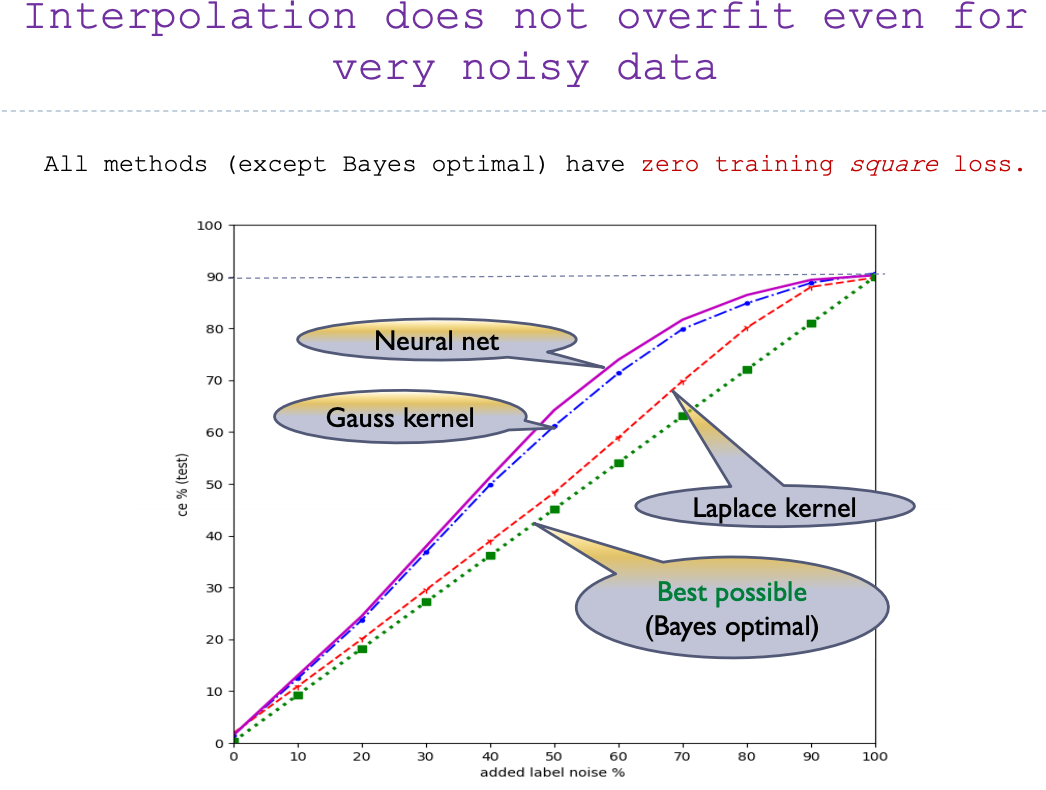
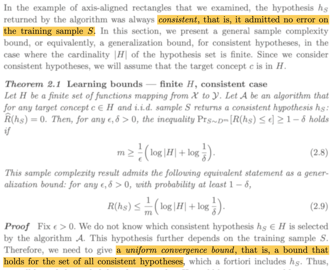
Interpolation learning Classical wisdom: “a model with zero training error is overfit to the training data and will typically generalize poorly”
(when
\lossdist(f^*) > 0
We'll call a model with
\losssamp(f) = 0
interpolating predictor
Added label noise on MNIST (%)
\lossdist(\hat f) \le \underbrace{\losssamp(\hat f)}_0 + \sqrt{\frac{C_{\mathcal F, \delta}}{n}}
\sqrt{\frac{C_{\mathcal F, \delta}}{n}}
Belkin/Ma/Mandal, ICML 2018
\sqrt{\frac{C_{\mathcal F, \delta}}{n}}
\lossdist(\hat f) \le {\color{#aaa} \losssamp(\hat f) +} \text{bound}
\lossdist(\hat f) \le \lossdist(f^*) + \text{bound}
*One exception-ish
[Negrea/Dziugaite/Roy, ICML 2020 ] :
\hat f
A more specific version of the question Today, we're mainly going to worry about consistency :
\E[ \lossdist(\hat f) - \lossdist(f^*)] \to 0
…in a noisy setting:
\lossdist(f^*) > 0
…for Gaussian linear regression:
\x \sim \N(\zero, \Sigma) \quad y = \langle \x, w^* \rangle + \N(\zero, \sigma^2) \quad L(y, \hat y) = (y - \hat y)^2
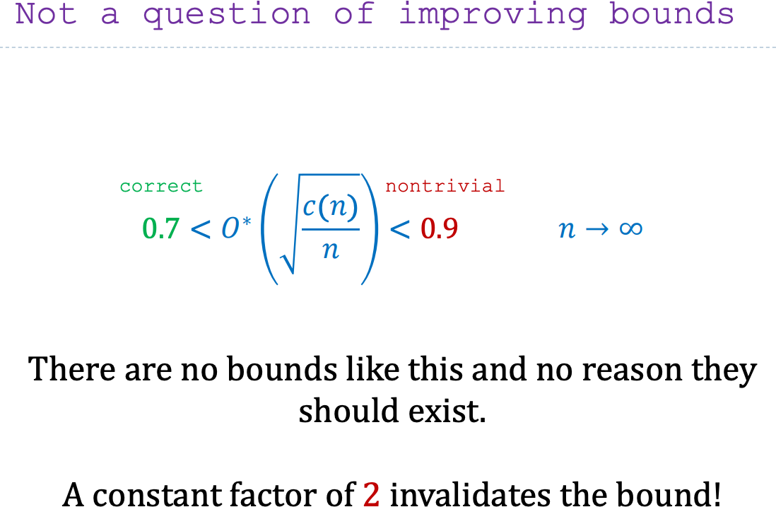
Is it possible to show consistency of an interpolator with
\lossdist(\hat f)
\le \underbrace{\losssamp(\hat f)}_0
+ \sup_{f \in \mathcal F} \left\lvert \lossdist(f) - \losssamp(f) \right\rvert
?
This requires tight constants!
A testbed problem: “junk features” “signal”,
\dS
“junk”,
\dJ \to \infty
\x
\x_S \sim \mathcal N\left( \zero_{d_S}, \eye_{d_S} \right)
\x_J \sim \mathcal N\left( \zero_{d_J}, \frac{\lambda_n}{d_J} \eye_{d_J} \right)
\w^*
\w_S^*
\zero
y = \underbrace{\langle \x, \w^* \rangle}_{\langle \xS, \wS^* \rangle} + \mathcal N(0, \sigma^2)
\lambda_n
\E \lVert \xJ \rVert_2^2 = \lambda_n
Linear regression:
\loss(y, \hat y) = (y - \hat y)^2
Min-norm interpolator:
\displaystyle \wmn = \argmin_{\X \w = \Y} \lVert \w \rVert_2 = \X^\dagger \Y
Consistency of
\wmn
\displaystyle \wmn = \argmin_{\X \w = \Y} \lVert \w \rVert_2 = \X^\dagger \Y
As
\dJ \to \infty
\wmn
\wmn
when
\dS
\dJ \to \infty
\lambda_n = o(n)
Could we have shown that with uniform convergence?
No uniform convergence on norm balls Theorem:
In junk features with
\lambda_n = o(n)
\lim_{n\to\infty} \lim_{\dJ \to \infty}
\E\left[ \sup_{\fragment[0][highlight-current-blue]{\norm\w_2 \le \norm\wmn_2}} \lvert \lossdist(\w) - \losssamp(\w) \rvert \right]
= \fragment[1][highlight-current-blue]{\infty}
.
No uniform convergence on norm balls - proof sketch Theorem:
In junk features with
\lambda_n = o(n)
\lim_{n\to\infty} \lim_{\dJ \to \infty}
\E\left[ \sup_{\fragment[0][highlight-current-blue]{\norm\w_2 \le \norm\wmn_2}} \lvert \lossdist(\w) - \losssamp(\w) \rvert \right]
= \fragment[1][highlight-current-blue]{\infty}
.
Proof idea:
\begin{align*}
\lossdist(\w)
&= (\w - \w^*)\tp \bSigma (\w - \w^*) + \lossdist(\w^*)
\\
\fragment[4]{ \lossdist(\w) - \losssamp(\w) }
&\fragment[4]{{}= (\w - \w^*) (\bSigma - \hat\bSigma) (\w - \w^*) }
\\&\quad \fragment[4]{
+ \left( \lossdist(\w^*) - \losssamp(\w^*) \right)
- \text{cross term}
}
\\
\fragment[5]{ \sup [\dots] }
&\fragment[5]{{}\ge \lVert \bSigma - \hat\bSigma \rVert_\op \cdot ( \norm\wmn_2 - \norm{\w^*}_2 )^2 + o(1) }
\fragment[9]{\to \infty}
\end{align*}
\Theta\left( \frac{n}{\lambda_n} \right)
\Theta\left( \sqrt{\frac{\lambda_n}{n}} \right)
Koltchinskii/Lounici, Bernoulli 2017
A more refined uniform convergence analysis?
\{ \w : \lVert\w\rVert \le B \}
Maybe
\{ \w : A \le \lVert\w\rVert \le B \}
In junk features,
for each
\delta \in (0, \frac12)
,
let
\Pr\left(\samp \in \mathcal{S}_{n,\delta}\right) \ge 1 - \delta
,
\hat\w
a
natural consistent interpolator,
and
\mathcal{W}_{n,\delta} = \left\{ \hat\w(\samp) : \samp \in \mathcal{S}_{n,\delta} \right\}
.
Then, almost surely,
\lim_{n \to \infty} \lim_{\dJ \to \infty}
\sup_{\samp \in \mathcal{S}_{n,\delta}}
%\E_{\samp} \left[
\sup_{\w \in \mathcal{W}_{n,\delta}}
\lvert \lossdist(\w) - \losssamp(\w) \rvert
%\right]
\ge 3 \sigma^2
.
([Negrea/Dziugaite/Roy, ICML 2020 ] had a very similar result for
\wmn
Natural interpolators:
\Scol{\hat\w_S}
\XJ
-\XJ
\wmn
\displaystyle \argmin_{\w:\X\w = \Y} \lVert \w \rVert_1
\displaystyle \argmin_{\w:\X\w = \Y} \lVert \w - \w^* \rVert_2
\displaystyle \argmin_{\w:\X\w = \Y} \Scol{f_S(\w_S)} + \Jcol{f_J(\w_J)}
f
\Jcol{f_J(-\w_J) = f_J(\w_J)}
Proof shows that for most
\samp
\w
\mathcal W_{n,\delta}
\lossdist(\w) \to \sigma^2
specifically
\samp
\losssamp(\w) \to 4 \sigma^2
So, what are we left with? Convergence of surrogates [Negrea/Dziugaite/Roy, ICML 2020 ] ?Nice, but not really the same thing… Only do analyses based on e.g. exact form of
\wmn
We'd like to keep good things about uniform convergence:Apply to more than just one specific predictor Tell us more about “why” things generalize Easier to apply without a nice closed form Or… One-sided uniform convergence? We don't really care about small
\lossdist
\losssamp
\sup \lossdist - \losssamp
\sup \lvert \lossdist - \losssamp \rvert
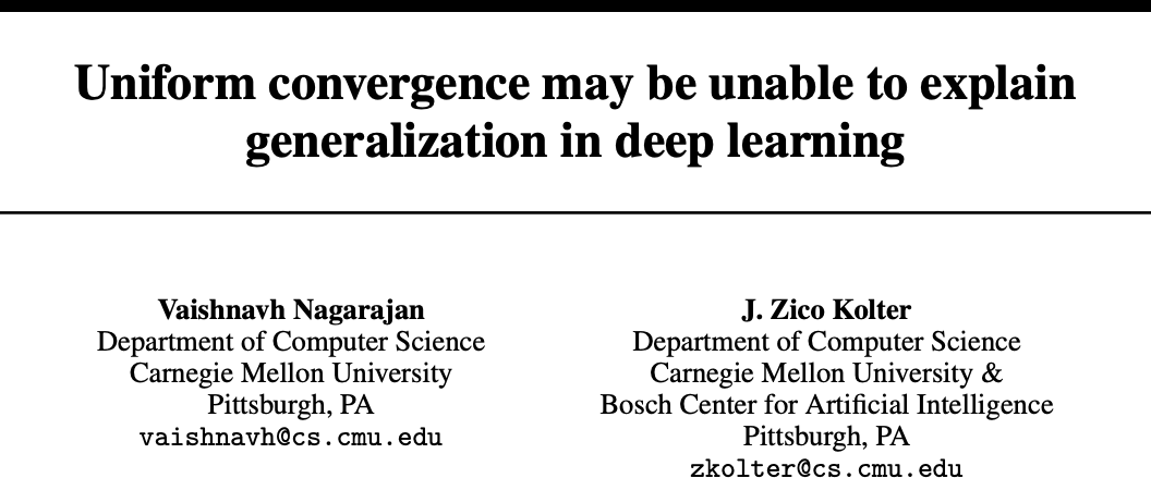
Existing uniform convergence proofs are “really” about
\lvert \lossdist - \losssamp \rvert
[Nagarajan/Kolter, NeurIPS 2019 ] Strongly expect still
\infty
\lambda_\max(\bSigma - \hat\bSigma)
\lVert \bSigma - \hat\bSigma \rVert_\op
Not possible to show
\sup_{f \in \mathcal F} \lossdist - \losssamp
all
\mathcal F
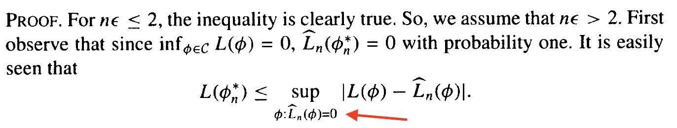
If
\hat f
\inf_f \losssamp(f) \ge 0
\mathcal F = \{ f : \lossdist(f) \le \lossdist(f^*) + \epsilon_{n,\delta} \}
A broader view of uniform convergence So far, used
\displaystyle
\lossdist(\w) - \losssamp(\w)
\le \sup_{\norm\w_2 \le B} \left\lvert \lossdist(\w) - \losssamp(\w) \right\rvert
But we only care about interpolators . How about
\sup_{\norm\w_2 \le B, \;\color{blue}{\losssamp(\w) = 0}} \left\lvert \lossdist(\w) \fragment[][highlight-gray]{- \losssamp(\w)} \right\rvert
?
Is this “uniform convergence”?
It's the standard notion for noiseless (
\lossdist(w^*) = 0
The interpolator ball in linear regression What does
\{\w :
\fragment[0][highlight-blue]{\norm\w_2 \le B}, \,
\fragment[1][highlight-red]{\losssamp(\w) = 0}
\}
\{ \w : \losssamp(\w) = \frac1n \lVert \X \w - \Y \rVert_2^2 = 0 \}
\X\w = \Y
Intersection of
d
with
(d-n)
:
(d-n)
centered at
\wmn
Optimistic rates Applying [Srebro/Sridharan/Tewari 2010 ] :
for all
\norm\w_2 \le B
\textstyle
\lossdist(\w) - \losssamp(\w)
\le \tilde{\bigO}_P\left( \frac{B^2 \psi_n}{n} + \sqrt{\losssamp(\w) \frac{B^2 \psi_n}{n} } \right)
\psi_n
\max_{i=1,\dots,n} \lVert \x_i \rVert_2^2
\sup_{\lVert\w\rVert_2 \le B,\, {\color{blue} \losssamp(\w) = 0 }}
\lossdist(\w)
\le {\color{red} c} \frac{B^2 \psi_n}{n} + o_P(1)
if
1 \ll \lambda_n \ll n
B = \lVert\wmn\rVert_2
\to c \lossdist(\w^*)
c \le 200,000 \, \log^3(n)
If this holds with
c = 1
(and maybe
\psi_n = \E \norm{\x}_2^2
,
B = \alpha \lVert\wmn\rVert_2
\alpha^2 \lossdist(\w^*)
Main result of first paper Theorem: If
\lambda_n = o(n)
\lim_{n \to \infty} \lim_{\dJ \to \infty} \E\left[
\sup_{\substack{\lVert\w\rVert \le \alpha \lVert\wmn\rVert\\\losssamp(\w) = 0}}
{\color{#aaa} \!\!\!\vert}\!\!\! \lossdist(\w) {\color{#aaa} {} - \losssamp(\w) \rvert}
\right]
\!= \alpha^2 \lossdist(\w^*)
Confirms speculation based on
\color{red} c = 1
Shows consistency with uniform convergence (of interpolators) New result for error of not-quite-minimal-norm interpolatorsNorm
\lVert\wmn\rVert + \text{const}
Norm
1.1 \lVert\wmn\rVert
1.21 \lossdist(\w^*)
What does
\{\w :
\fragment[0][highlight-blue]{\lVert\w\rVert \le B}, \,
\fragment[1][highlight-red]{\losssamp(\w) = 0}
\}
\{ \w : \losssamp(\w) = \frac1n \lVert \X \w - \Y \rVert^2 = 0 \}
\X\w = \Y
Intersection of
d
with
(d-n)
:
(d-n)
centered at
\wmn
Can write as
\{\hat\w + \F \z : \z \in \R^{d-n},\, \lVert \hat\w + \F \z \rVert \le B \}
\hat\w
any interpolator,
\F
\operatorname{ker}(\X)
Decomposition via strong duality Can change variables in
\sup_{\w : \lVert \w \rVert \le B, \, \losssamp(\w) = 0} \lossdist(\w)
\lossdist(\w^*) +
\sup_{\z : \lVert \hat\w + \F \z \rVert^2 \le B^2}
(\hat\w + \F \z - w^*)\tp \bSigma (\hat\w + \F \z - w^*)
Quadratic program, one quadratic constraint: strong duality
Exactly equivalent to problem in one scalar variable:
\lossdist(\hat{\w})
+ \inf_{\mu > \lVert \F\tp \bSigma \F \rVert }
\left\lVert \F\tp [ \mu \hat{\w} - \Sigma(\hat{\w} - \w^*)] \right\rVert_{
(\mu \eye_{p-n} - \F\tp \bSigma \F)^{-1}
}
+ \mu (B^2 - \lVert \hat{\w} \rVert^2)
Can analyze this for different choices of
\hat\w
The minimal-risk interpolator
\begin{align*}
\wmr \,
&{}= \argmin_{\w : \X \w = \Y} \lossdist(\w)
\\&\fragment{= \w^* + \Sigma^{-1} \X\tp (\X \Sigma^{-1} \X\tp)^{-1} (Y - X \w^*)}
\end{align*}
In Gaussian least squares generally, have that
\E \lossdist(\wmr) = \frac{d - 1}{d - 1 - n} \lossdist(\w^*)
\wmr
n = o(d)
Very useful for lower bounds! [Muthukumar+ JSAIT 2020 ]
Restricted eigenvalue under interpolation
\kappa_\X(\bSigma)
= \sup_{\lVert\w\rVert = 1, \; \X\w = \zero} \w\tp \bSigma \w
Roughly, “how much” of
\bSigma
\X
Consistency up to
\lVert\wmr\rVert
Analyzing dual with
\wmr
,
get without
any distributional assumptions that
\sup_{\substack{\lVert\w\rVert \le \lVert\wmr\rVert\\\losssamp(\w) = 0}} \lossdist(\w)
= \lossdist(\wmr) + \beta \, \kappa_X(\Sigma) \left[ \lVert\wmr\rVert^2 - \lVert\wmn\rVert^2 \right]
(amount of missed energy)
\cdot
(available norm)
If
\wmr
consistent, everything smaller-norm also consistent iff
\beta
term
\to 0
In our setting:
\wmr
is consistent,
\lossdist(\wmr) \to \lossdist(\w^*)
\kappa_X(\bSigma) \approx \frac{\lambda_n}{n}
\quad
\E\left[ \lVert\wmr\rVert^2 - \lVert\wmn\rVert^2 \right]
= \frac{\sigma^2 d_S}{\lambda_n} + o\left(1\right)
Plugging in:
\quad
\E \sup_{\lVert\w\rVert \le \lVert\wmr\rVert,\, \losssamp(\w) = 0} \lossdist(\w)
\to \lossdist(\w^*)
In the generic results,
\lossdist
\lossdist(\w) = \lossdist(\w^*) + (\w - \w^*)\tp \Sigma (\w - \w^*)
\w^*
Error up to
\alpha \lVert\wmn\rVert
Analyzing dual with
\wmn
\hat\w
\alpha \ge 1
\sup_{\substack{\lVert\w\rVert \le \alpha \lVert\wmn\rVert \\\losssamp(\w) = 0}} \lossdist(\w)
= \lossdist(\wmn) + (\alpha^2 - 1) \, \kappa_X(\Sigma) \, \lVert\wmn\rVert^2 + R_n
R_n \to 0
\wmn
In our setting:
\wmn
\lVert\wmn\rVert \le \lVert\wmr\rVert
\E \kappa_\X(\bSigma) \, \lVert\wmn\rVert^2 \to \sigma^2 = \lossdist(\w^*)
Plugging in:
\quad \E \sup_{\lVert\w\rVert \le \alpha \lVert\wmn\rVert,\, \losssamp(\w) = 0} \lossdist(\w) \to \alpha^2 \lossdist(\w^*)
…and we're done!
Conjecture holds (for Gaussian linear regression) Specifically, our more general bound implies that w.h.p.
\sup_{\norm{\w}_2 \le B, \, \losssamp(\w) = 0} \lossdist(\w)
\le (1 + o(1)) \frac{B^2 \Tr(\Sigma_2)}{n}
\Sigma = \Sigma_1 \oplus \Sigma_2
\Tr(\Sigma_2) \le \Tr(\Sigma) = \E \norm\x^2
For this to mean anything, need
B \ge \wmn
Combine with a new analysis on
\norm\wmn
\norm\wmn_2 \le \norm{\w^*}_2 + (1 + o(1)) \; \sqrt{\frac{\sigma^2 n}{\Tr(\Sigma_2)}}
Benign overfitting of
\wmn
Plugging the two bounds together:
\lossdist(\hat\w) \le (1 + o(1)) \left( \sigma + \norm{\w^*} \sqrt{\frac{\Tr(\Sigma_2)}{n}} \right)^2
Including all the fiddly conditions I didn't mention, [Bartlett/Long/Lugosi/Tsigler PNAS 2020 ]
Additionally tells us about nearly-minimal-norm interpolators
Generalization error in compact sets Theorem .
If
\Sigma = \Sigma_1 \oplus \Sigma_2
with
\operatorname{rank}(\Sigma_1) = o(n)
,
w.h.p.
\sup_{\w \in \K, \, \losssamp(\w) = 0} \lossdist(\w)
\le (1 + o(1)) \, \frac{W(\Sigma_2^{1/2} \mathcal K)^2}{n}
W(\K) := \E_{H \sim \N(\zero, \eye_d)} \left[ \sup_{\w \in \K} \lvert\langle H, \w \rangle\rvert \right]
this is an informal statement, but gets the gist
Norm needed to interpolate for general norms Theorem .
Let
\norm\cdot_*
\norm\cdot
\hat\w = \argmin_{\w : \losssamp(\w) = 0} \norm\w
Under some conditions, w.h.p.
\norm{\hat\w}
\le \norm{\w^*} + (1 + o(1)) \frac{\sigma \sqrt{n}}{\E_{H \sim \N(\zero, \eye_d)} \norm{\Sigma_2^{1/2} H}_*}
.
Plugging them together,
get consistency conditions analogous to the [BLLT] ones
for minimal-norm interpolators for any norm.
New application: minimum
\norm\w_1
LASSO, Adaboost, compressed sensing, basis pursuit, …
Much harder to analyze directly, because no closed form!
[Ju/Lin/Liu NeurIPS 2020 ]
[Chinot/Löffler/van de Geer 2021 ]
Our conditions hold in a junk features setting, if
d = e^{\omega(n)}
Very limited setting, but (as far as we know)
\sigma > 0
w^* \ne \zero
On Uniform Convergence and Low-Norm Interpolation Learning
Zhou, Sutherland, Srebro
NeurIPS 2020
Uniform Convergence of Interpolators:
Koehler*, Zhou*, Sutherland, Srebro
NeurIPS 2021
Junk features example:
\wmn
Uniform convergence over norm ball can't show any learning Uniform convergence of interpolators does workMatches previously known (nearly necessary) sufficient conditions Applies to general norm balls (though can be hard to evaluate) Our analysis is very specific to Gaussian data Coming soon : extension to near-interpolators via optimistic rates