Better GANs by Using Kernels
Mikołaj Bińkowski
Imperial
![]()
![]()
UMass Amherst, Sep 30 2019
(Swipe or arrow keys to move through slides; m for a menu to jump; ? for help.
Vertical slides are backups that I probably won't show in the talk.)
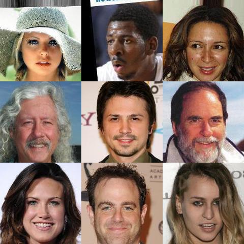
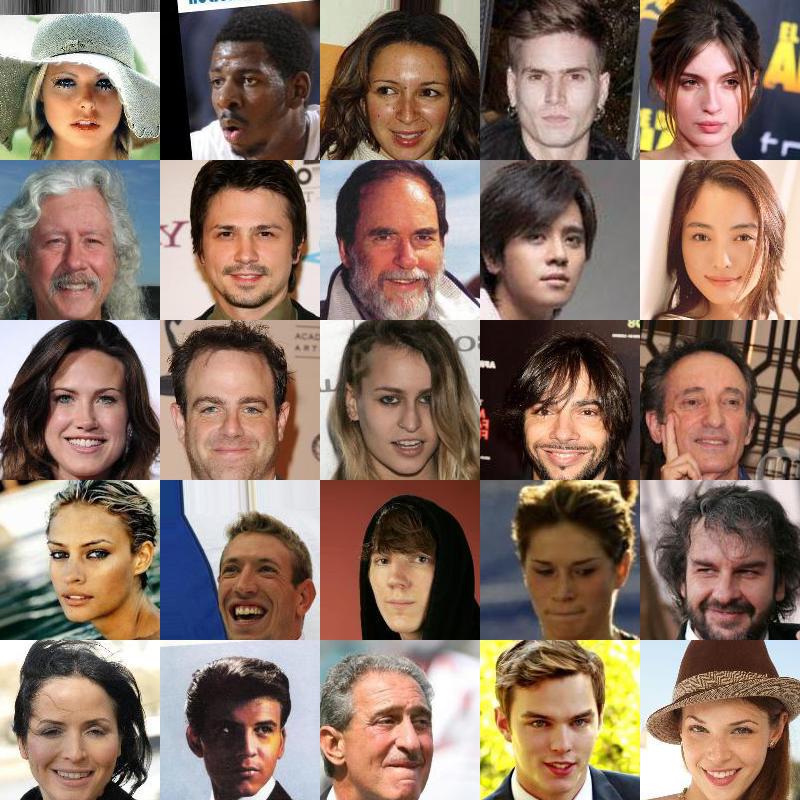
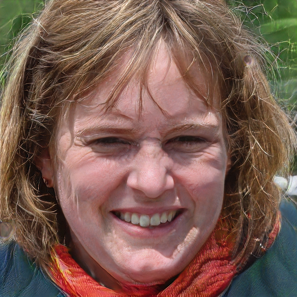
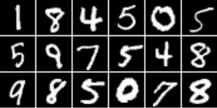
Implicit generative models
Given samples from a distribution over ,
we want a model that can produce new samples from
![]()
![]()
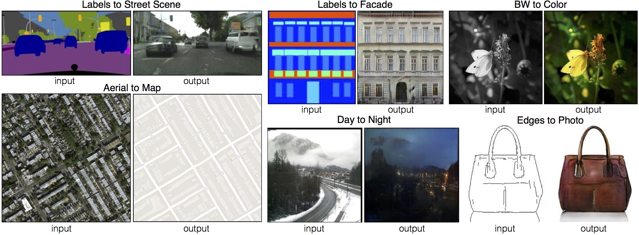
Why implicit generative models?
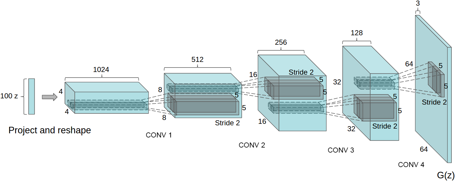
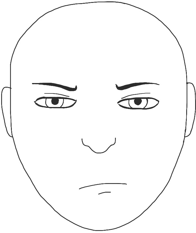
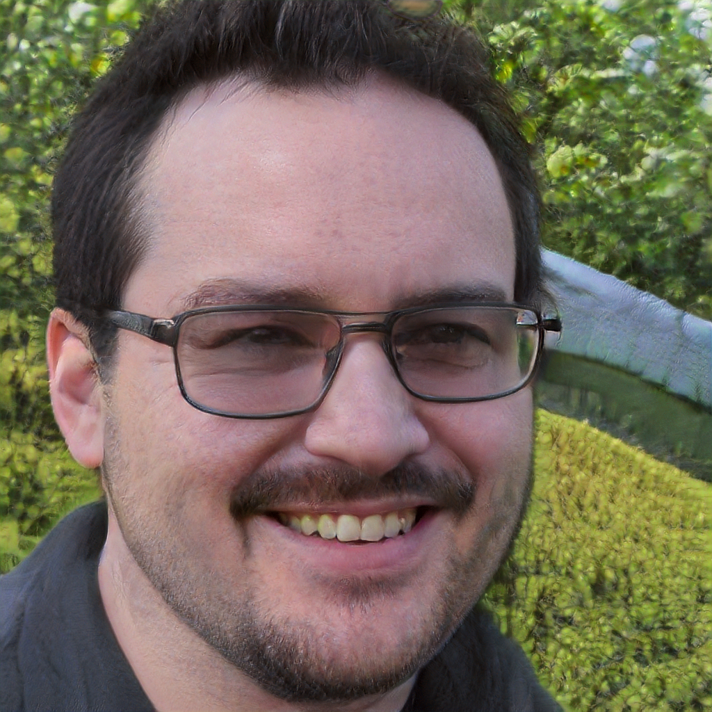
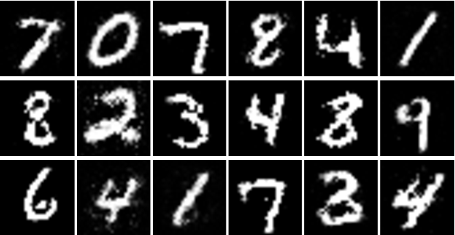
How to generate images things?
One choice: with a generator!
Fixed distribution of latents:
Maps through a network:
![]()
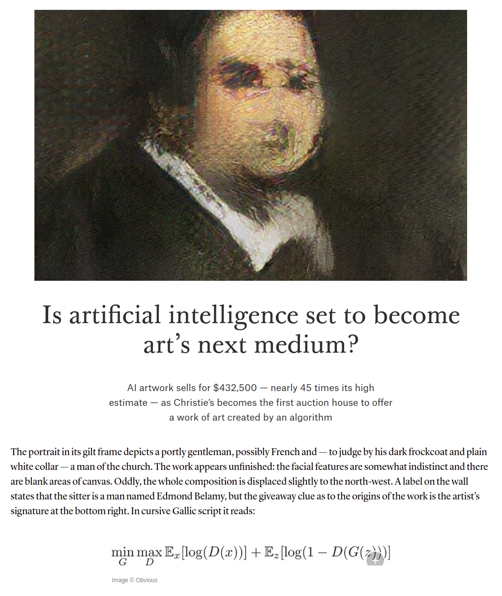
How to choose ?
Generator ()
![]()
Discriminator
![]()
Target ()
![]()
Is this real?![]()
No way!
:( I'll try harder…
⋮
Is this real?![]()
Umm…
One view: distances between distributions
- What happens when is at its optimum?
- If distributions have densities,
- If stays optimal throughout, tries to minimize
which is
- If and have (almost) disjoint support
so
Discriminator point of view
Generator ()
![]()
Discriminator
![]()
Target ()
![]()
Is this real?![]()
No way!
:( I don't know how to do any better…
How likely is disjoint support?
- At initialization, pretty reasonable:
:
![]()
:
![]()
- Remember we might have
- For usual , is supported on a countable union of
manifolds with dim - “Natural image manifold” usually considered low-dim
- No chance that they'd align at init, so
Path to a solution: integral probability metrics
is a critic function
Total variation:
Wasserstein:
Maximum Mean Discrepancy [Gretton+ 2012]
Kernel – a “similarity” function
For many kernels, iff
MMD as feature matching
- is the feature map for
- If , ;
MMD is distance between means
- Many kernels: infinite-dimensional
Derivation of MMD
Reproducing property: if ,
Estimating MMD
- No need for a discriminator – just minimize !
- Continuous loss, gives “partial credit”
Generator ()
![]()
Critic
![]()
Target ()
![]()
How are these?![]()
![]()
![]()
Not great!
:( I'll try harder…
⋮
Deep kernels
![]()
- usually Gaussian, linear, …
MMD loss with a deep kernel
- from pretrained Inception net
- simple: exponentiated quadratic or polynomial
![]()
![]()
- Don't just use one kernel, use a class parameterized by :
- New distance based on all these kernels:
- Minimax optimization problem
Non-smoothness of Optimized MMD
Illustrative problem in , DiracGAN [Mescheder+ ICML-18]:
- Just need to stay away from tiny bandwidths
- …deep kernel analogue is hard.
- Instead, keep witness function from being too steep
- would give Wasserstein
- Nice distance, but hard to estimate
- Control on average, near the data
MMD GANs versus WGANs
- Linear- MMD GAN, :
- WGAN has:
- We were just trying something like an unregularized WGAN…
MMD-GAN with gradient control
- If gives uniformly Lipschitz critics, is smooth
- Original MMD-GAN paper [Li+ NeurIPS-17]: box constraint
- We [Bińkowski+ ICLR-18] used gradient penalty on critic instead
- Better in practice, but doesn't fix the Dirac problem…
New distance: Scaled MMD
Want to ensure
Can do directly with kernel properties…but too expensive!
Guaranteed if
Gives distance
Deriving the Scaled MMD
Constraint can be written
Smoothness of
Theorem: is continuous.
If has a density; is Gaussian/linear/…;
is fully-connected, Leaky-ReLU, non-increasing width;
all weights in have bounded condition number; then
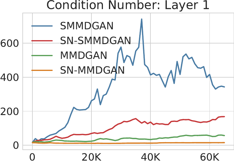
Keeping weight condition numbers bounded
- Spectral parameterization [Miyato+ ICLR-18]:
- ; learn and freely
- Encourages diversity without limiting representation
![]()
Rank collapse
- Occasional optimization failure without spectral param:
- Generator doing reasonably well
- Critic filters become low-rank
- Generator corrects it by breaking everything else
- Generator gets stuck
What if we just did spectral normalization?
- , so that ,
- Works well for original GANs [Miyato+ ICLR-18]
- …but doesn't work at all as only constraint in a WGAN
- Limits representation too much
- In DiracGAN, only allows bandwidth 1
Continuity theorem proof
- means
- Can show
- By assumption on ,
- Because Leaky-ReLU, ,
- For Lebesgue-almost all ,
: 2d example
Target
and model
samples
![]()
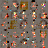
Kernels from
, early in optimization
![]()
Kernels from
(early)
![]()
Critic gradients from
(early)
![]()
Critic gradients from
(early)
![]()
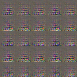
Kernels from
,
late in optimization
![]()
Kernels from
(late)
![]()
Critic gradients from
(late)
![]()
Critic gradients from
(late)
![]()
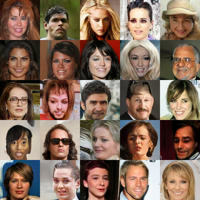
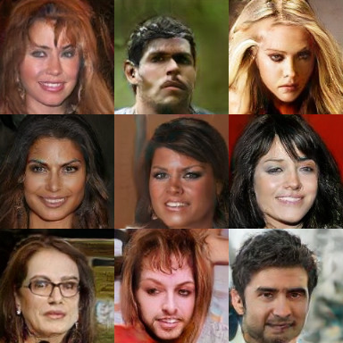
Model on CelebA
SN-SMMD-GAN
![]()
KID: 0.006
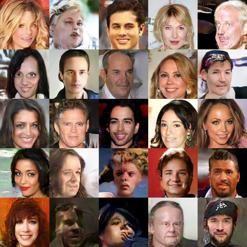
WGAN-GP
![]()
KID: 0.022
Implicit generative model evaluation
- No likelihoods, so…how to compare models?
- Main approach:
look at a bunch of pictures and see if they're pretty or not- Easy to find (really) bad samples
- Hard to see if modes are missing / have wrong probabilities
- Hard to compare models beyond certain threshold
- Need better, quantitative methods
- Our method: Kernel Inception Distance (KID)
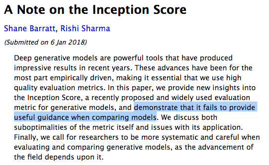
- Previously standard quantitative method
- Based on ImageNet classifier label predictions
- Classifier should be confident on individual images
- Predicted labels should be diverse across sample
- No notion of target distribution
- Scores completely meaningless on LSUN, Celeb-A, SVHN, …
- Not great on CIFAR-10 either
![]()
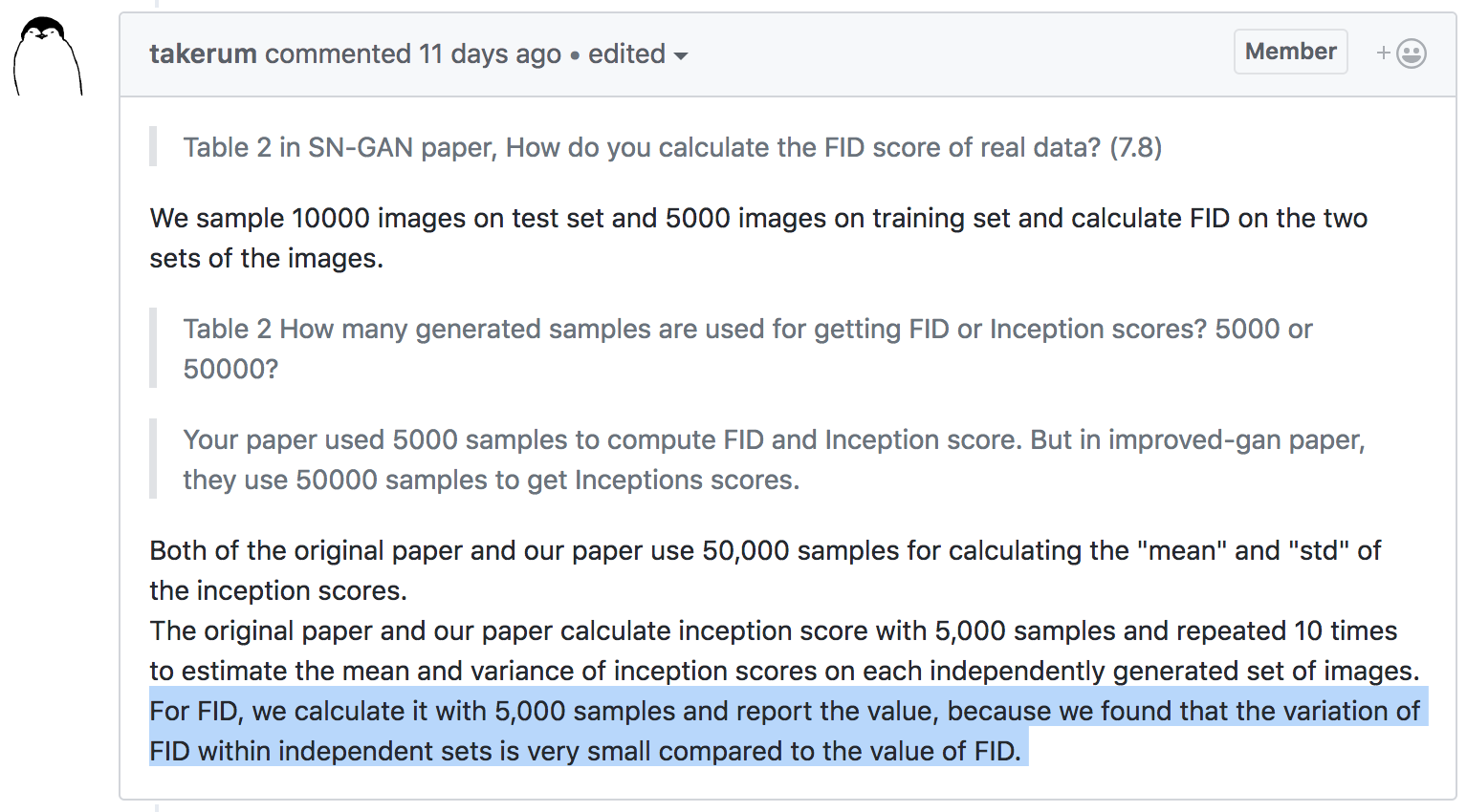
Fréchet Inception Distance (FID) [Heusel+ NIPS-17]
- Fit normals to Inception hidden layer activations of and
- Compute Fréchet (Wasserstein-2) distance between fits
- Meaningful on not-ImageNet datasets
- Estimator extremely biased, tiny variance
- ,
![]()
New method: Kernel Inception Distance (KID)
![]()
Automatic learning rate adaptation with KID
- Models need appropriate learning rate schedule to work well
- Automate with three-sample MMD test [Bounliphone+ ICLR-16]:
![]()
Training process on CelebA
Controlling critic complexity
![]()
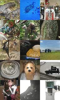
Model on ImageNet
SN-SMMDGAN
![]()
KID: 0.035
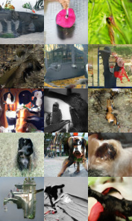
SN-GAN
![]()
KID: 0.044
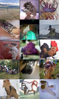
BGAN
![]()
KID: 0.047
Recap
- Can train generative models by minimizing
a flexible, smooth distance between distributions
- Combine kernels with gradient penalties
- Strong practical results, some understanding of theory
Demystifying MMD GANs
Bińkowski*, Sutherland*, Arbel, and Gretton
ICLR 2018
On Gradient Regularizers for MMD GANs
Arbel*, Sutherland*, Bińkowski, and Gretton
NeurIPS 2018
Links + code: see djsutherland.ml. Thanks!
Learning deep kernels for exponential family densities
Wenliang*, Sutherland*, Strathmann, and Gretton
ICML 2019


.svg)
.svg)
.svg)
.svg)
.svg)
.svg)
.svg)
.svg)