Deep kernel-based distances between distributions
Danica J. Sutherland
Based on work with:Michael Arbel
Mikołaj Bińkowski
Soumyajit De
Arthur Gretton
Feng Liu
Jie Lu
Aaditya Ramdas
Alex Smola
Heiko Strathmann
Hsiao-Yu (Fish) Tung
Wenkai Xu
Guangquan Zhang
![]()
![]()
PIHOT kick-off, 30 Jan 2021
(Swipe or arrow keys to move through slides; for a menu to jump; to show more.)
What's a kernel again?
- Linear classifiers: ,
- Use a “richer” :
- Can avoid explicit ; instead
- “Kernelized” algorithms access data only through
Reproducing Kernel Hilbert Space (RKHS)
- Ex: Gaussian RBF / exponentiated quadratic / squared exponential / …
- Reproducing property: for
- ,
where
-
is in
– the representer theorem
Maximum Mean Discrepancy (MMD)
MMD as feature matching
- is the feature map for
- If , ;
MMD is distance between means
- Many kernels: infinite-dimensional
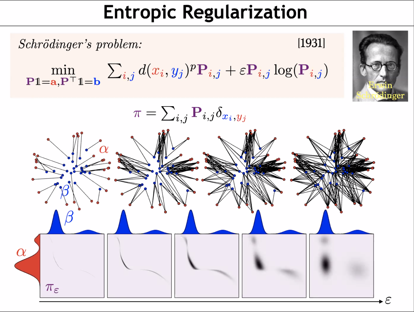
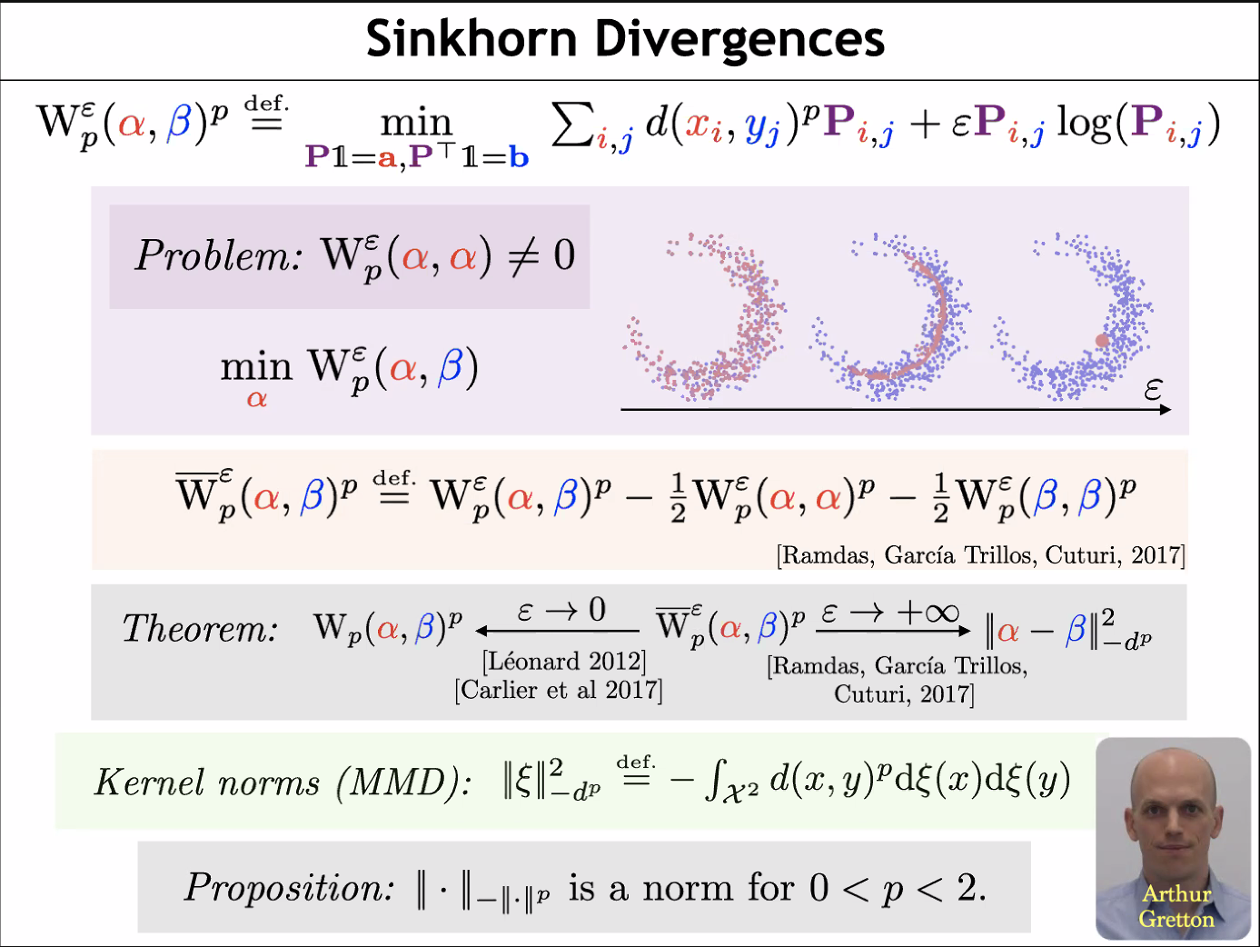
MMD and OT
![]()
![]()
Estimating MMD
I: Two-sample testing
- Given samples from two unknown distributions
- Question: is ?
- Hypothesis testing approach:
- Reject if test statistic
- Do smokers/non-smokers get different cancers?
- Do Brits have the same friend network types as Americans?
- When does my laser agree with the one on Mars?
- Are storms in the 2000s different from storms in the 1800s?
- Does presence of this protein affect DNA binding? [MMDiff2]
- Do these dob and birthday columns mean the same thing?
- Does my generative model match ?
- Independence testing: is ?
What's a hypothesis test again?
Permutation testing to find
Need
: th quantile of
MMD-based tests
- If is characteristic, iff
- Efficient permutation testing for
- : converges in distribution
- : asymptotically normal
- Any characteristic kernel gives consistent test…eventually
- Need enormous if kernel is bad for problem
Classifier two-sample tests
![]()
- is the accuracy of on the test set
- Under , classification impossible:
- With where ,
get
Optimizing test power
- Asymptotics of give us immediately that
, , are constants:
first term dominates
- Pick to maximize an estimate of
- Can show uniform convergence of estimator
Blobs dataset
![]()
Blobs results
![]()
CIFAR-10 vs CIFAR-10.1
Train on 1 000, test on 1 031, repeat 10 times. Rejection rates:| ME | SCF | C2ST | MMD-O | MMD-D |
|---|
| 0.588 | 0.171 | 0.452 | 0.316 | 0.744 |
Ablation vs classifier-based tests
| Cross-entropy | Max power |
|---|
| Dataset | Sign | Lin | Ours | Sign | Lin | Ours |
|---|
| Blob | 0.84 | 0.94 | 0.90 | – | 0.95 | 0.99 |
|---|
| High- Gauss. mix. | 0.47 | 0.59 | 0.29 | – | 0.64 | 0.66 |
|---|
| Higgs | 0.26 | 0.40 | 0.35 | – | 0.30 | 0.40 |
|---|
| MNIST vs GAN | 0.65 | 0.71 | 0.80 | – | 0.94 | 1.00 |
|---|
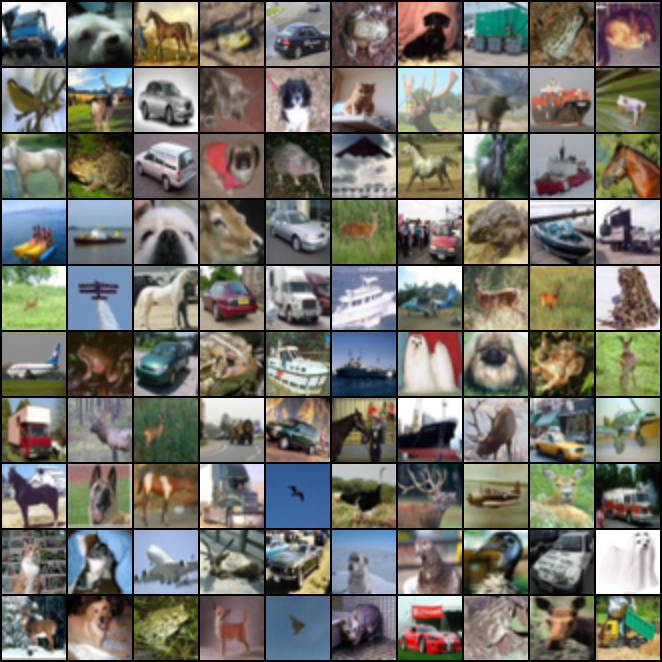
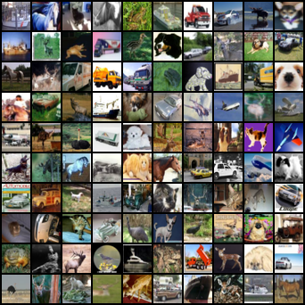
II: Training implicit generative models
Given samples from a distribution over ,
we want a model that can produce new samples from
![]()
![]()
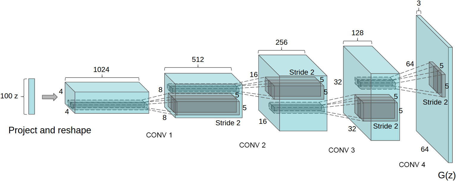
Generator networks
Fixed distribution of latents:
Maps through a network:
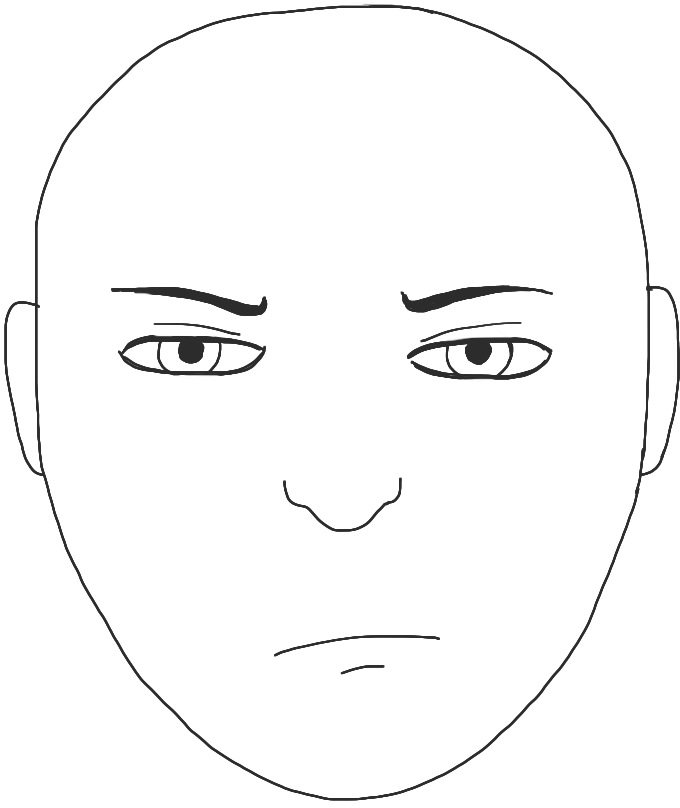
![]()
DCGAN generator [Radford+ ICLR-16]
How to choose ?
GANs and their flaws
- GANs [Goodfellow+ NeurIPS-14] minimize discriminator accuracy (like classifier test) between and
- Problem: if there's a perfect classifier, discontinuous loss, no gradient to improve it [Arjovsky/Bottou ICLR-17]
Disjoint at init:
:
![]()
:
![]()
- For usual , is supported on a countable union of manifolds with dim
- “Natural image manifold” usually considered low-dim
- Won't align at init, so won't ever align
WGANs and MMD GANs
- Integral probability metrics with “smooth” are continuous
- WGAN: a set of neural networks satisfying
- WGAN-GP: instead penalize near the data
- Both losses are MMD with
- Some kind of constraint on is important!
Non-smoothness of plain MMD GANs
Illustrative problem in , DiracGAN [Mescheder+ ICML-18]:
- Just need to stay away from tiny bandwidths
- …deep kernel analogue is hard.
- Instead, keep witness function from being too steep
- would give Wasserstein
- Nice distance, but hard to estimate
- Control on average, near the data
MMD-GAN with gradient control
- If gives uniformly Lipschitz critics, is smooth
- Original MMD-GAN paper [Li+ NeurIPS-17]: box constraint
- We [Bińkowski+ ICLR-18] used gradient penalty on critic instead
- Better in practice, but doesn't fix the Dirac problem…
New distance: Scaled MMD
Want to ensure
Can solve with …but too expensive!
Guaranteed if
Gives distance
Deriving the Scaled MMD
Smoothness of
Theorem: is continuous.
If has a density;
is Gaussian/linear/…;
is fully-connected, Leaky-ReLU, non-increasing width;
all weights in have bounded condition number;
then
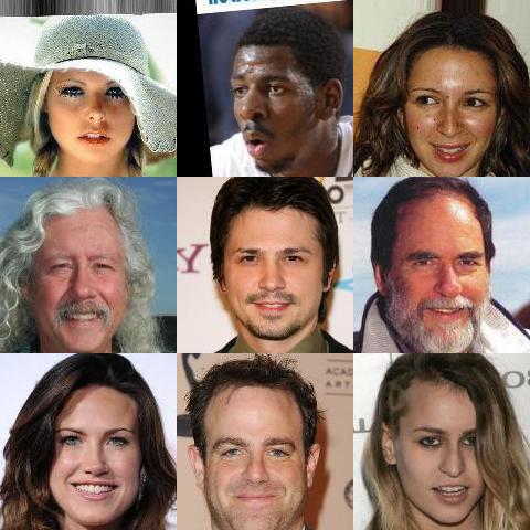
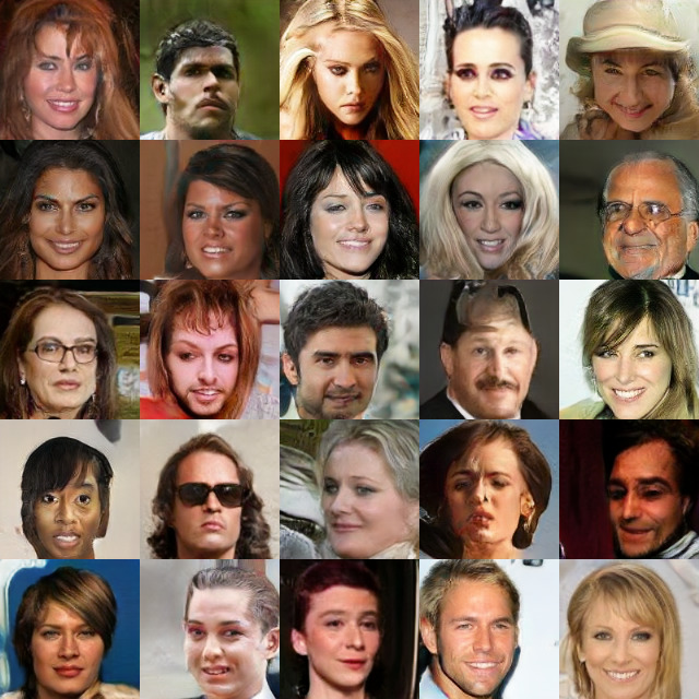
Results on CelebA
SN-SMMD-GAN
![]()
KID: 0.006
WGAN-GP
![]()
KID: 0.022
Training process on CelebA
Evaluating generative models
![]()
Evaluating generative models
- Human evaluation: good at precision, bad at recall
- Likelihood: hard for GANs, maybe not right thing anyway
- Two-sample tests: always reject!
- Most common: Fréchet Inception Distance, FID
- Run pretrained featurizer on model and target
- Model each as Gaussian; compute
- Strong bias, small variance: very misleading
- Simple examples where
but
for reasonable sample size
- Our KID: instead. Unbiased, asymptotically normal
Recap
Combining a deep architecture with a kernel machine that takes the higher-level learned representation as input can be quite powerful.
— Y. Bengio & Y. LeCun (2007), “Scaling Learning Algorithms towards AI”
- Two-sample testing [ICLR-17, ICML-20]
- Choose to maximize power criterion
- Exploit closed form of for permutation testing
- Generative modeling with MMD GANs [ICLR-18, NeurIPS-18]
- Need a smooth loss function for the generator
- Better gradients for generator to follow (?)
Future uses of deep kernel distances
- Selective inference to avoid train/test split? Meta-testing?
- When , can we tell how they're different?
- Methods so far: some mostly for low-
- Some look at points with large critic function
- Does model match dataset (Stein testing)?
- Maximize deep dependence measure for unsupervised representation learning, as in contrastive learning
- …


 KID: 0.006
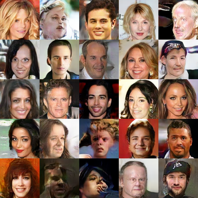 KID: 0.022