\definecolor{cb1}{RGB}{76,114,176} \definecolor{cb2}{RGB}{221,132,82} \definecolor{cb3}{RGB}{85,168,104} \definecolor{cb4}{RGB}{196,78,82} \definecolor{cb5}{RGB}{129,114,179} \definecolor{cb6}{RGB}{147,120,96} \definecolor{cb7}{RGB}{218,139,195} \DeclareMathOperator*{\argmin}{argmin} \DeclareMathOperator*{\argmax}{argmax} \newcommand{\bigO}{\mathcal{O}} \newcommand{\bigO}{\mathcal{O}} \newcommand{\bSigma}{\mathbf{\Sigma}} \newcommand{\D}{\mathcal{D}} \DeclareMathOperator*{\E}{\mathbb{E}} \newcommand{\eye}{\mathbf{I}} \newcommand{\F}{\mathbf{F}} \newcommand{\Lip}{\mathrm{Lip}} \DeclareMathOperator{\loss}{\mathit{L}} \DeclareMathOperator{\lossdist}{\loss_\D} \DeclareMathOperator{\losssamp}{\loss_\samp} \newcommand{\samp}{\mathbf{S}} \newcommand{\R}{\mathbb{R}} \newcommand{\tp}{^{\mathsf{T}}} \newcommand{\w}{\mathbf{w}} \newcommand{\wmn}{\hat{\w}_{\mathit{MN}}} \newcommand{\wmr}{\hat{\w}_{\mathit{MR}}} \newcommand{\x}{\mathbf{x}} \newcommand{\X}{\mathbf{X}} \newcommand{\Y}{\mathbf{y}} \newcommand{\y}{\mathrm{y}} \newcommand{\z}{\mathbf{z}} \newcommand{\zero}{\mathbf{0}} \newcommand{\Scol}[1]{{\color{cb1} #1}} \newcommand{\Jcol}[1]{{\color{cb2} #1}} \newcommand{\dS}{\Scol{d_S}} \newcommand{\dJ}{\Jcol{d_J}} \newcommand{\xS}{\Scol{\x_S}} \newcommand{\xJ}{\Jcol{\x_J}} \newcommand{\XS}{\Scol{\X_S}} \newcommand{\XJ}{\Jcol{\X_J}} \newcommand{\wS}{\Scol{\w_S}} \newcommand{\wsS}{\Scol{\w_S^*}} \newcommand{\wJ}{\Jcol{\w_J}} \newcommand{\wlam}{\Scol{\hat{\w}_{\lambda_n}}}

Can Uniform Convergence
Explain Interpolation Learning?

D.J. Sutherland
TTI-Chicago → UBC
based on arXiv:2006.05942 (NeurIPS 2020), with:
Lijia Zhou
U Chicago
Nati Srebro
TTI-Chicago

Penn State Statistics Seminar, October 8 2020

(Swipe or arrow keys to move through slides; m for a menu to jump; ? to show more.)

Supervised learning

  • Given i.i.d. samples \samp = \{(\x_i, y_i)\}_{i=1}^n \sim \D^n
    • features/covariates \x_i \in \R^d , labels/targets y_i \in \R
  • Want f such that f(\x) \approx y for new samples from \D : f^* = \argmin\left[ \lossdist(f) := \E_{(\x, \y) \sim \D} \loss(f(\x), \y) \right]
    • e.g. squared loss: L(\hat y, y) = (\hat y - y)^2
  • Standard approaches based on empirical risk minimization: \hat{f} \approx \argmin\left[ \losssamp(f) := \frac1n \sum_{i=1}^n \loss(f(\x_i), y_i) \right]

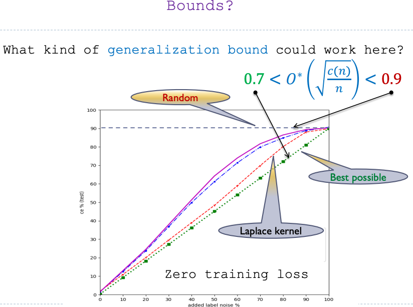
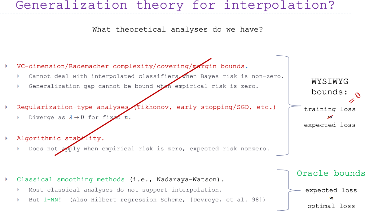
Statistical learning theory

We have lots of bounds like: with probability \ge 1 - \delta , \sup_{f \in \mathcal F} \left\lvert \lossdist(f) - \losssamp(f) \right\rvert \le \sqrt{ \frac{C_{\mathcal F, \delta}}{n} }

C_{\mathcal F,\delta} could be from VC dimension, covering number, RKHS norm, Rademacher complexity, fat-shattering dimension, …

Then for large n , \lossdist(f) \approx \losssamp(f) , so \hat f \approx f^*

\lossdist(\hat f) \le \losssamp(\hat f) + \sup_{f \in \mathcal F} \left\lvert \lossdist(f) - \losssamp(f) \right\rvert

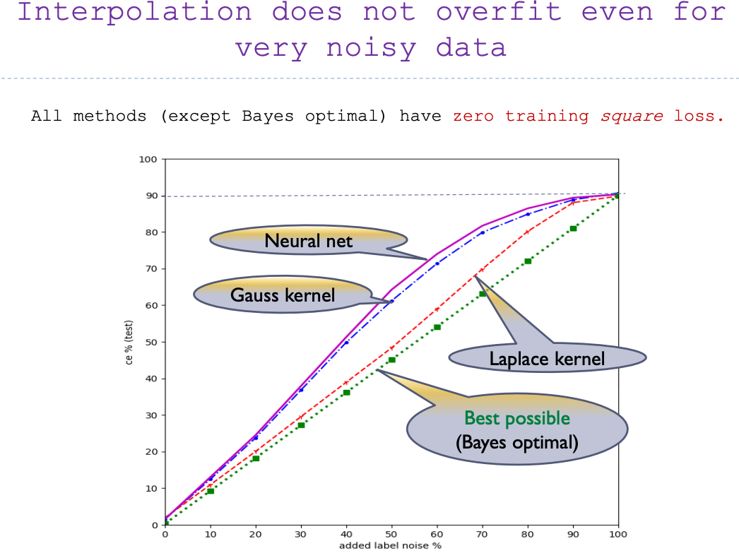
Interpolation learning

Classical wisdom: “a model with zero training error is overfit to the training data and will typically generalize poorly”
(when \lossdist(f^*) > 0 )
\losssamp(\hat f) = 0 ; \lossdist(\hat f) \approx 11\% Zhang et al., “Rethinking generalization”, ICLR 2017

We'll call a model with \losssamp(f) = 0 an interpolating predictor

Misha Belkin
Simons Institute
July 2019
\losssamp(\hat f) = 0
f^*
\lossdist(f)
Added label noise on MNIST (%)
Belkin/Ma/Mandal, ICML 2018
Misha Belkin
Simons Institute
July 2019
\lossdist(f)
Added label noise on MNIST (%)
\lossdist(\hat f) \le \underbrace{\losssamp(\hat f)}_0 + \sqrt{\frac{C_{\mathcal F, \delta}}{n}}
\sqrt{\frac{C_{\mathcal F, \delta}}{n}}
Belkin/Ma/Mandal, ICML 2018
Misha Belkin
Simons Institute
July 2019
\sqrt{\frac{C_{\mathcal F, \delta}}{n}}
Misha Belkin
Simons Institute
July 2019
\lossdist(\hat f) \le {\color{#aaa} \losssamp(\hat f) +} \text{bound}
\lossdist(\hat f) \le \lossdist(f^*) + \text{bound}

Lots of recent theoretical work on interpolation.
[Belkin+ NeurIPS 2018], [Belkin+ AISTATS 2018], [Belkin+ 2019], [Hastie+ 2019],
[Muthukumar+ JSAIT 2020], [Bartlett+ PNAS 2020], [Liang+ COLT 2020], [Montanari+ 2019], many more…

None* bound \sup_{f \in \mathcal F} \lvert \lossdist(f) - \losssamp(f) \rvert .
Is it possible to find such a bound?
Can uniform convergence explain interpolation learning?

*One exception-ish [Negrea/Dziugaite/Roy, ICML 2020]:
relates \hat f to a surrogate predictor,
shows uniform convergence for the surrogate

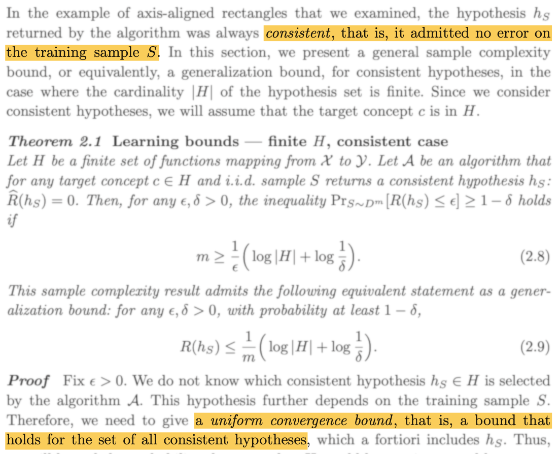
A more specific version of the question

We're only going to worry about consistency: \E[ \lossdist(\hat f) - \lossdist(f^*)] \to 0

…in a non-realizable setting: \lossdist(f^*) > 0

Is it possible to show consistency of an interpolator with \lossdist(\hat f) \le \underbrace{\losssamp(\hat f)}_0 + \sup_{f \in \mathcal F} \left\lvert \lossdist(f) - \losssamp(f) \right\rvert ?

This requires tight constants!

Our testbed problem

“signal”, \dS “junk”, \dJ \to \infty
\x \x_S \sim \mathcal N\left( \zero_{d_S}, \eye_{d_S} \right) \x_J \sim \mathcal N\left( \zero_{d_J}, \frac{\lambda_n}{d_J} \eye_{d_J} \right)
\w^* \w_S^* \zero
y = \underbrace{\langle \x, \w^* \rangle}_{\langle \xS, \wS^* \rangle} + \mathcal N(0, \sigma^2)

\lambda_n controls scale of junk: \E \lVert \xJ \rVert^2 = \lambda_n

Linear regression: \loss(y, \hat y) = (y - \hat y)^2

Min-norm interpolator: \displaystyle \wmn = \argmin_{\X \w = \Y} \lVert \w \rVert_2 = \X^\dagger \Y

Consistency of \wmn

As \dJ \to \infty , \wmn approaches ridge regression on the signal: \displaystyle \langle \wmn, \x \rangle \stackrel{\dJ \to \infty}{\longrightarrow} \langle \wlam, \xS \rangle for almost all \x

\displaystyle \wlam = \argmin_{\wS \in \R^{\dS}} \lVert \Scol{\X_S \w_S}^2 - \Y \rVert^2 + \lambda_n \lVert \wS \rVert^2

If \lambda_n = o(n) , \wlam is consistent: \lossdist(\wlam) \stackrel{n \to \infty}{\longrightarrow} \sigma^2

\wmn is consistent when \dS fixed, \dJ \to \infty , \lambda_n = o(n) .

Could we have shown that with uniform convergence?

No uniform convergence on norm balls

Theorem: If \lambda_n = o(n) , \lim_{n\to\infty} \lim_{\dJ \to \infty} \E\left[ \sup_{\fragment[0][highlight-current-blue]{\lVert\w\rVert \le \lVert\wmn\rVert}} \lvert \lossdist(\w) - \losssamp(\w) \rvert \right] = \fragment[1][highlight-current-blue]{\infty} .

Proof idea:

\begin{align*} \lossdist(\w) &= (\w - \w^*)\tp \bSigma (\w - \w^*) + \lossdist(\w^*) \\ \fragment[4]{ \lossdist(\w) - \losssamp(\w) } &\fragment[4]{{}= (\w - \w^*) (\bSigma - \hat\bSigma) (\w - \w^*) } \\&\quad \fragment[4]{ + \left( \lossdist(\w^*) - \losssamp(\w^*) \right) - \text{cross term} } \\ \fragment[5]{ \sup [\dots] } &\fragment[5]{{}\ge \lVert \bSigma - \hat\bSigma \rVert \cdot ( \lVert\wmn\rVert - \lVert\w^*\rVert )^2 + o(1) } \fragment[9]{\to \infty} \end{align*}

\Theta\left( \frac{n}{\lambda_n} \right) \Theta\left( \sqrt{\frac{\lambda_n}{n}} \right)
Koltchinskii/Lounici, Bernoulli 2017

A more refined uniform convergence analysis?

\{ \w : \lVert\w\rVert \le B \} is no good. Maybe \{ \w : A \le \lVert\w\rVert \le B \} ?

Theorem (à la [Nagarajan/Kolter, NeurIPS 2019]):
For each \delta \in (0, \frac12) , let \Pr\left(\samp \in \mathcal{S}_{n,\delta}\right) \ge 1 - \delta ,
\hat\w a natural consistent interpolator,
and \mathcal{W}_{n,\delta} = \left\{ \hat\w(\samp) : \samp \in \mathcal{S}_{n,\delta} \right\} . Then, almost surely,
\lim_{n \to \infty} \lim_{\dJ \to \infty} \sup_{\samp \in \mathcal{S}_{n,\delta}} %\E_{\samp} \left[ \sup_{\w \in \mathcal{W}_{n,\delta}} \lvert \lossdist(\w) - \losssamp(\w) \rvert %\right] \ge 3 \sigma^2 .

([Negrea/Dziugaite/Roy, ICML 2020] had a very similar result for \wmn )

Natural interpolators: \Scol{\hat\w_S} doesn't change if \XJ flips to -\XJ . Examples:
\wmn , \displaystyle \argmin_{\w:\X\w = \Y} \lVert \w \rVert_1 , \displaystyle \argmin_{\w:\X\w = \Y} \lVert \w - \w^* \rVert_2 ,
\displaystyle \argmin_{\w:\X\w = \Y} \Scol{f_S(\w_S)} + \Jcol{f_J(\w_J)} with each f convex, \Jcol{f_J(-\w_J) = f_J(\w_J)}

Proof shows that for most \samp ,
there's a typical predictor \w (in \mathcal W_{n,\delta} )
that's good on most inputs ( \lossdist(\w) \to \sigma^2 ),
but very bad on specifically \samp ( \losssamp(\w) \to 4 \sigma^2 )

So, what are we left with?

One-sided uniform convergence?

We don't really care about small \lossdist , big \losssamp ….
Could we bound \sup \lossdist - \losssamp instead of \sup \lvert \lossdist - \losssamp \rvert ?

  • Existing uniform convergence proofs are “really” about \lvert \lossdist - \losssamp \rvert [Nagarajan/Kolter, NeurIPS 2019]
  • Strongly expect still \infty for norm balls in our testbed
    • \lambda_\max(\bSigma - \hat\bSigma) instead of \lVert \bSigma - \hat\bSigma \rVert
  • Not possible to show \sup_{f \in \mathcal F} \lossdist - \losssamp is big for all \mathcal F
    • If \hat f consistent and \inf_f \losssamp(f) \ge 0 , use \mathcal F = \{ f : \lossdist(f) \le \lossdist(f^*) + \epsilon_{n,\delta} \}

A broader view of uniform convergence

So far, used \displaystyle \lossdist(\w) - \losssamp(\w) \le \sup_{\lVert\w\rVert \le B} \left\lvert \lossdist(\w) - \losssamp(\w) \right\rvert

But we only care about interpolators. How about \sup_{\lVert\w\rVert \le B, \;\color{blue}{\losssamp(\w) = 0}} \left\lvert \lossdist(\w) \fragment[][highlight-gray]{- \losssamp(\w)} \right\rvert ?

Is this “uniform convergence”?

It's the standard notion for realizable ( \lossdist(w^*) = 0 ) analyses…

Are there analyses like this for \lossdist(w^*) > 0 ?

Optimistic rates

Applying [Srebro/Sridharan/Tewari 2010]: for all \lVert\w\rVert \le B , \textstyle \lossdist(\w) - \losssamp(\w) \le \tilde{\bigO}_P\left( \frac{B^2 \xi_n}{n} + \sqrt{\losssamp(\w) \frac{B^2 \xi_n}{n} } \right) \xi_n : high-prob bound on \max_{i=1,\dots,n} \lVert \x_i \rVert^2

\sup_{\lVert\w\rVert \le B,\, {\color{blue} \losssamp(\w) = 0 }} \lossdist(\w) \le {\color{red} c} \frac{B^2 \xi_n}{n} + o_P(1)

if 1 \ll \lambda_n \ll n , B = \lVert\wmn\rVert , \to c \lossdist(\w^*)
c \le 200,000 \, \log^3(n)

But if we suppose c = 1 , would get a novel prediction: \sup_{\lVert\w\rVert \le \alpha \lVert\wmn\rVert,\, \losssamp(\w) = 0} \lossdist(\w) \le \alpha^2 \left[ \sigma^2 + o_P(1) \right]

Main result

Theorem: If \lambda_n = o(n) , \lim_{n \to \infty} \lim_{\dJ \to \infty} \E\left[ \sup_{\substack{\lVert\w\rVert \le \alpha \lVert\wmn\rVert\\\losssamp(\w) = 0}} {\color{#aaa} \!\!\!\vert}\!\!\! \lossdist(\w) {\color{#aaa} {} - \losssamp(\w) \rvert} \right] \!= \alpha^2 \lossdist(\w^*)

  • Confirms speculation based on \color{red} c = 1 assumption
  • Shows consistency with uniform convergence (of interpolators)
  • New result for error of not-quite-minimal-norm interpolators
    • Norm \lVert\wmn\rVert + \text{const} is asympotically consistent
    • Norm 1.1 \lVert\wmn\rVert is at worst 1.21 \lossdist(\w^*)

What does \{\w : \fragment[0][highlight-blue]{\lVert\w\rVert \le B}, \, \fragment[1][highlight-red]{\losssamp(\w) = 0} \} look like?

\{ \w : \losssamp(\w) = \frac1n \lVert \X \w - \Y \rVert^2 = 0 \} is the plane \X\w = \Y

Intersection of d -ball with (d-n) -hyperplane:
(d-n) -ball centered at \wmn

Can write as \{\hat\w + \F \z : \z \in \R^{d-n},\, \lVert \hat\w + \F \z \rVert \le B \}
where \hat\w is any interpolator, \F is basis for \operatorname{ker}(\X)

Decomposition via strong duality

Can change variables in \sup_{\w : \lVert \w \rVert \le B, \, \losssamp(\w) = 0} \lossdist(\w) to \lossdist(\w^*) + \sup_{\z : \lVert \hat\w + \F \z \rVert^2 \le B^2} (\hat\w + \F \z - w^*)\tp \bSigma (\hat\w + \F \z - w^*)

Quadratic program, one quadratic constraint: strong duality

Exactly equivalent to problem in one scalar variable: \lossdist(\hat{\w}) + \inf_{\mu > \lVert \F\tp \bSigma \F \rVert } \left\lVert \F\tp [ \mu \hat{\w} - \Sigma(\hat{\w} - \w^*)] \right\rVert_{ (\mu \eye_{p-n} - \F\tp \bSigma \F)^{-1} } + \mu (B^2 - \lVert \hat{\w} \rVert^2)

Can analyze this for different choices of \hat\w

The minimal-risk interpolator

\begin{align*} \wmr \, &{}= \argmin_{\w : \X \w = \Y} \lossdist(\w) \\&\fragment{= \w^* + \Sigma^{-1} \X\tp (\X \Sigma^{-1} \X\tp)^{-1} (Y - X \w^*)} \end{align*}

In Gaussian least squares generally, have that \E \lossdist(\wmr) = \frac{d - 1}{d - 1 - n} \lossdist(\w^*) so \wmr is consistent iff n = o(d) .

Very useful for lower bounds! [Muthukumar+ JSAIT 2020]

Restricted eigenvalue under interpolation

\kappa_\X(\bSigma) = \sup_{\lVert\w\rVert = 1, \; \X\w = \zero} \w\tp \bSigma \w

Roughly, “how much” of \bSigma is “missed” by \X

Consistency up to \lVert\wmr\rVert

Analyzing dual with \wmr ,
get without any distributional assumptions that \sup_{\substack{\lVert\w\rVert \le \lVert\wmr\rVert\\\losssamp(\w) = 0}} \lossdist(\w) = \lossdist(\wmr) + \beta \, \kappa_X(\Sigma) \left[ \lVert\wmr\rVert^2 - \lVert\wmn\rVert^2 \right]
1 \le \beta \le 4
(amount of missed energy) \cdot (available norm)
If \wmr consistent, everything smaller-norm also consistent iff \beta term \to 0

In our setting:

\wmr is consistent, \lossdist(\wmr) \to \lossdist(\w^*)
\kappa_X(\bSigma) \approx \frac{\lambda_n}{n} \quad \E\left[ \lVert\wmr\rVert^2 - \lVert\wmn\rVert^2 \right] = \frac{\sigma^2 d_S}{\lambda_n} + o\left(1\right)
Plugging in: \quad \E \sup_{\lVert\w\rVert \le \lVert\wmr\rVert,\, \losssamp(\w) = 0} \lossdist(\w) \to \lossdist(\w^*)
In the generic results, \lossdist means \lossdist(\w) = \lossdist(\w^*) + (\w - \w^*)\tp \Sigma (\w - \w^*) for some \w^*

Error up to \alpha \lVert\wmn\rVert

Analyzing dual with \wmn for \hat\w , \alpha \ge 1 , get in general: \sup_{\substack{\lVert\w\rVert \le \alpha \lVert\wmn\rVert \\\losssamp(\w) = 0}} \lossdist(\w) = \lossdist(\wmn) + (\alpha^2 - 1) \, \kappa_X(\Sigma) \, \lVert\wmn\rVert^2 + R_n R_n \to 0 if \wmn is consistent

In our setting:

\wmn is consistent, because \lVert\wmn\rVert \le \lVert\wmr\rVert

\E \kappa_\X(\bSigma) \, \lVert\wmn\rVert^2 \to \sigma^2 = \lossdist(\w^*)

Plugging in: \quad \E \sup_{\lVert\w\rVert \le \alpha \lVert\wmn\rVert,\, \losssamp(\w) = 0} \lossdist(\w) \to \alpha^2 \lossdist(\w^*)

…and we're done!

On Uniform Convergence and Low-Norm Interpolation Learning
Zhou, Sutherland, and Srebro
NeurIPS 2020
  • “Regular” uniform convergence can't explain consistency of \wmn
    • Uniform convergence over norm ball can't show any learning
  • An “interpolating” uniform convergence bound does
    • Shows low norm is sufficient for interpolation learning here
    • Predicts exact worst-case error as norm grows
  • Optimistic/interpolating rates might be able to explain interpolation learning more broadly
    • Need to get the constants on leading terms exactly right!
  • Analyzing generalization gap via duality may be broadly applicable
    • Can always get upper bounds via weak duality