Better deep learning (sometimes)
by learning kernel mean embeddings
Danica J. Sutherland(she/her)University of British Columbia (UBC) / Alberta Machine Intelligence Institute (Amii)
slides (but not the talk) about four related projects:
![]()
Feng Liu
Wenkai Xu
Hsiao-Yu (Fish) Tung
(+ 6 more…)
![]()
Yazhe Li
Roman Pogodin
![]()
Michael Arbel
Mikołaj Bińkowski
![]()
Li (Kevin) Wenliang
Heiko Strathmann
+ all with Arthur Gretton
LIKE22 - 12 Jan 2022
(Swipe or arrow keys to move through slides; for a menu to jump; to show more.)
Deep learning and deep kernels
- Deep learning: models usually of form
- With a learned
- If we fix , have with
- Same idea as NNGP approximation
- Could train a classifier by:
- Let , loss of the best
- Learn by following
- Generalize to a deep kernel:
Normal deep learning deep kernels
- Take as output of last layer
- Final function in will be
- With logistic loss: this is Platt scaling
![]()
So what?
- This definitely does not say that deep learning is (even approximately) a kernel method
- …despite what some people might want you think
![]()
- We know theoretically deep learning can learn some things faster than any kernel method [see Malach+ ICML-21 + refs]
- But deep kernel learning ≠ traditional kernel models
- exactly like how usual deep learning ≠ linear models
What do deep kernels give us?
- In “normal” classification: slightly richer function space 🤷
- Meta-learning: common , constantly varying
- Two-sample testing
- Simple form of for cheap permutation testing
- Self-supervised learning
- Better understanding of what's really going on, at least
- Generative modeling with MMD GANs
- Better gradient for generator to follow (?)
- Score matching in exponential families (density estimation)
- Optimize regularization weights, better gradient (?)
Maximum Mean Discrepancy (MMD)
MMD as feature matching
- is the feature map for
- If , , then
the MMD is distance between means - Many kernels: infinite-dimensional
Estimating MMD
I: Two-sample testing
- Given samples from two unknown distributions
- Question: is ?
- Hypothesis testing approach:
- Reject if test statistic
- Do smokers/non-smokers get different cancers?
- Do Brits have the same friend network types as Americans?
- When does my laser agree with the one on Mars?
- Are storms in the 2000s different from storms in the 1800s?
- Does presence of this protein affect DNA binding? [MMDiff2]
- Do these dob and birthday columns mean the same thing?
- Does my generative model match ?
- Independence testing: is ?
What's a hypothesis test again?
Permutation testing to find
Need
: th quantile of
MMD-based tests
- If is characteristic, iff
- Efficient permutation testing for
- : converges in distribution
- : asymptotically normal
- Any characteristic kernel gives consistent test…eventually
- Need enormous if kernel is bad for problem
Classifier two-sample tests
![]()
- is the accuracy of on the test set
- Under , classification impossible:
- With where ,
get
Optimizing test power
- Asymptotics of give us immediately that
, , are constants:
first term dominates
- Pick to maximize an estimate of
- Can show uniform convergence of estimator
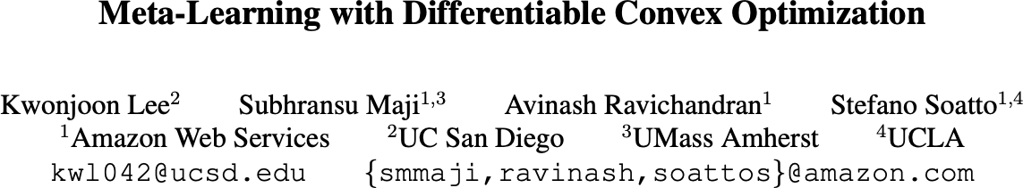
Blobs dataset
![]()
Blobs results
![]()
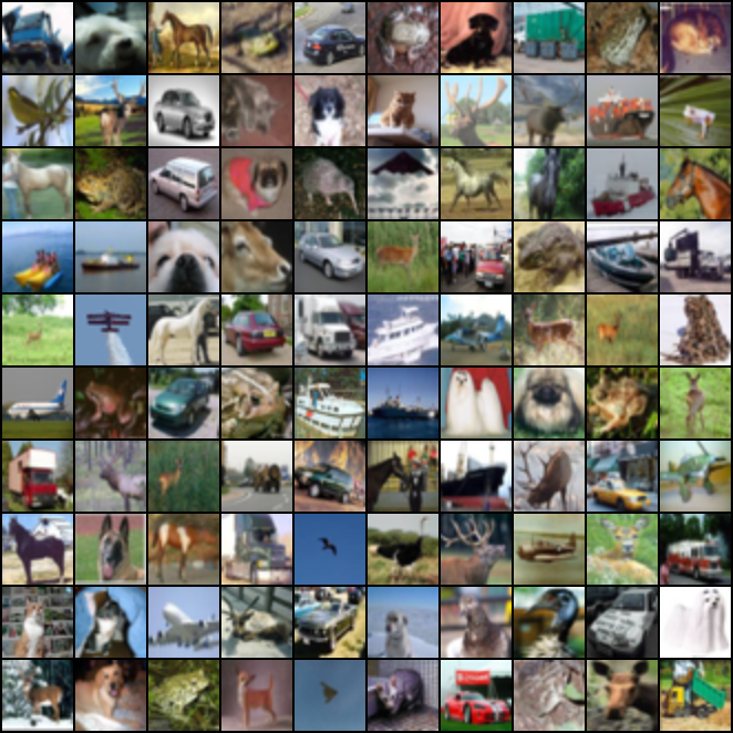
CIFAR-10 vs CIFAR-10.1
Train on 1 000, test on 1 031, repeat 10 times. Rejection rates:| ME | SCF | C2ST | MMD-O | MMD-D |
|---|
| 0.588 | 0.171 | 0.452 | 0.316 | 0.744 |
Ablation vs classifier-based tests
| Cross-entropy | Max power |
|---|
| Dataset | Sign | Lin | Ours | Sign | Lin | Ours |
|---|
| Blobs | 0.84 | 0.94 | 0.90 | – | 0.95 | 0.99 |
|---|
| High- Gauss. mix. | 0.47 | 0.59 | 0.29 | – | 0.64 | 0.66 |
|---|
| Higgs | 0.26 | 0.40 | 0.35 | – | 0.30 | 0.40 |
|---|
| MNIST vs GAN | 0.65 | 0.71 | 0.80 | – | 0.94 | 1.00 |
|---|
But…
- What if you don't have much data for your testing problem?
- Need enough data to pick a good kernel
- Also need enough test data to actually detect the difference
- Best split depends on best kernel's quality / how hard to find
- Don't know that ahead of time; can't try more than one
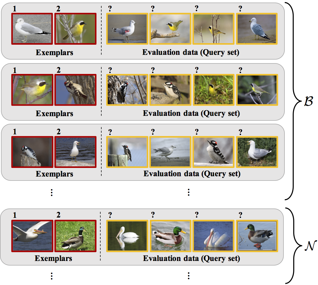
Meta-testing
- One idea: what if we have related problems?
- Similar setup to meta-learning:
![]() (from Wei+ 2018)
(from Wei+ 2018)
Meta-testing for CIFAR-10 vs CIFAR-10.1
- CIFAR-10 has 60,000 images, but CIFAR-10.1 only has 2,031
- Where do we get related data from?
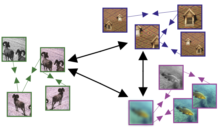
- One option: set up tasks to distinguish classes of CIFAR-10 (airplane vs automobile, airplane vs bird, ...)
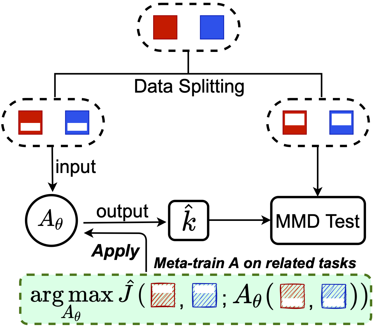
One approach (MAML-like)
![]()
is, e.g., 5 steps of gradient descent
we learn the initialization, maybe step size, etc
![]()
This works, but not as well as we'd hoped…
Initialization might work okay on everything, not really adapt
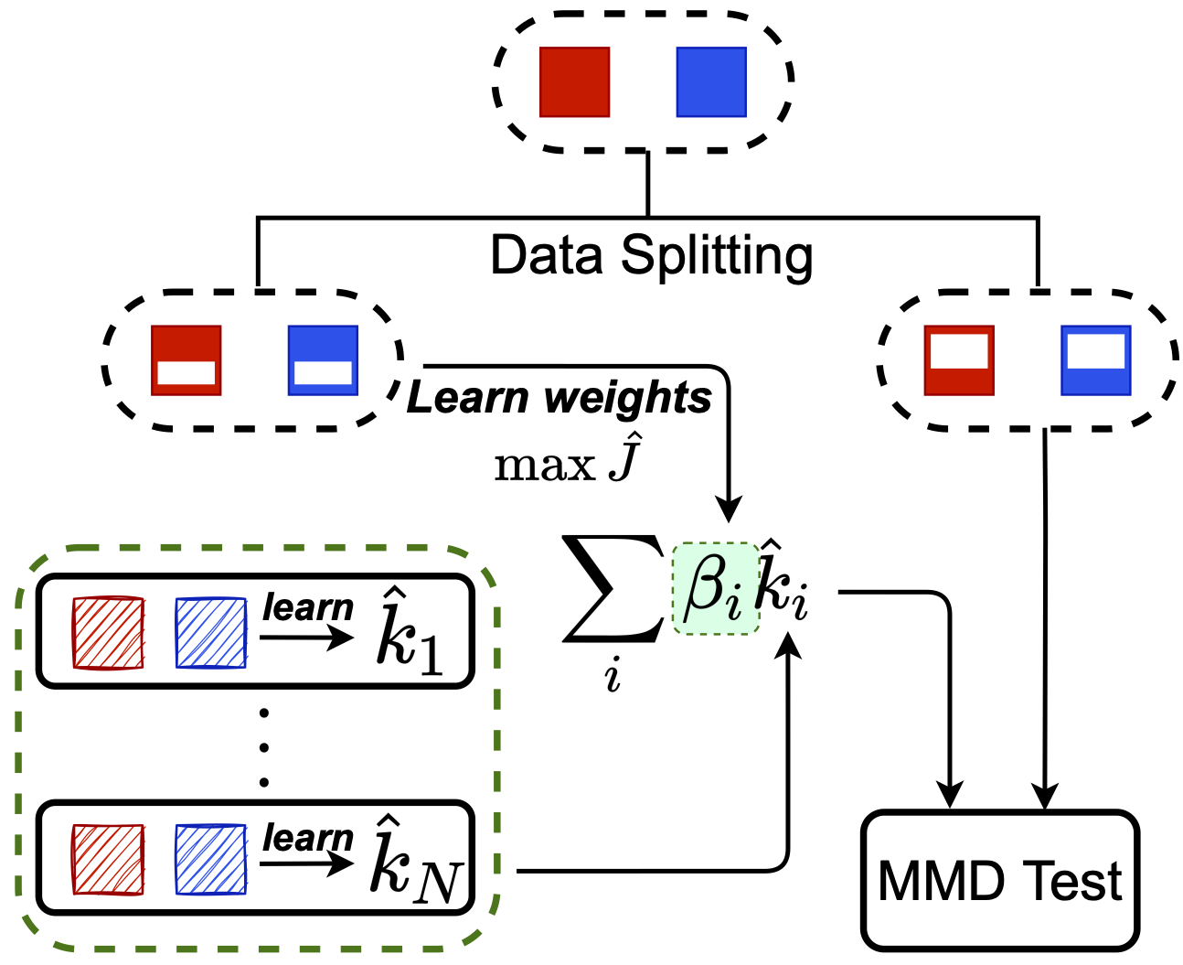
Another approach: Meta-MKL
![]()
Inspired by classic multiple kernel learning
Only need to learn linear combination
on test task:
much easier
![]()
Theoretical analysis for Meta-MKL
- Same big-O dependence on test task size 😐
- But multiplier is much better:
based on number of meta-training tasks, not on network size - (Analysis assumes meta-tasks are “related” enough)
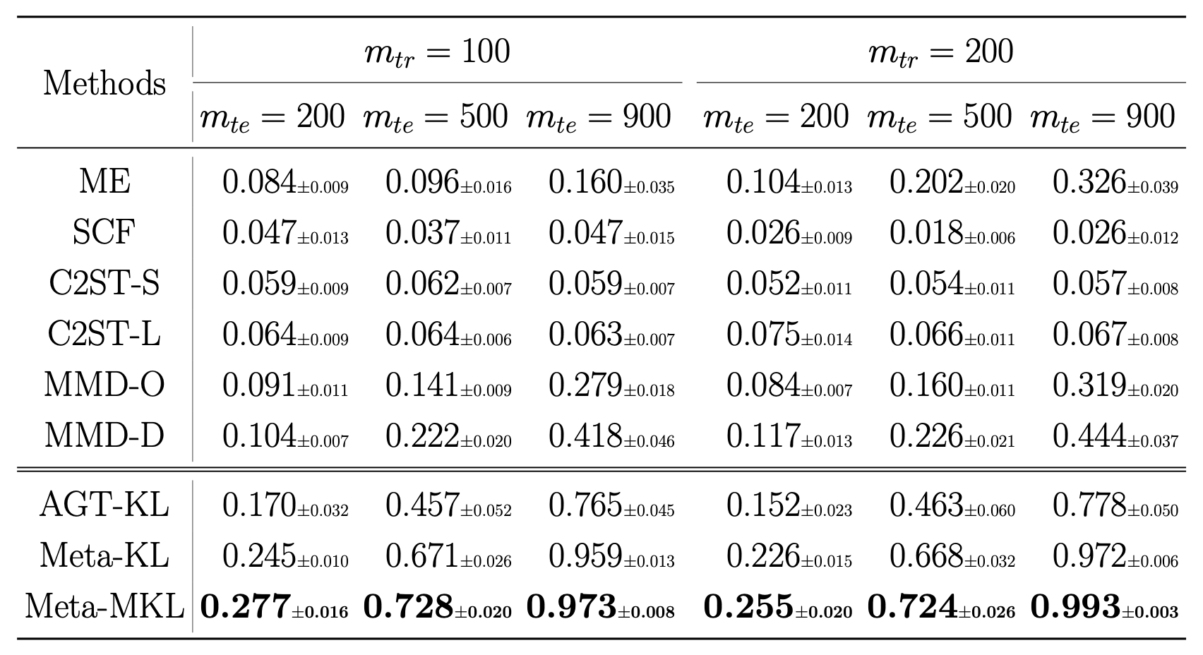
Results on CIFAR-10.1
![]()
Challenges for testing
- When , can we tell how they're different?
- Methods so far: some mostly for low-
- Some look at points with large critic function
- Finding kernels / features that can't do certain things
- distinguish by emotion, but can't distinguish by skin color
- Avoid the need for data splitting (selective inference)
- Kübler+ NeurIPS-20 gave one method
- only for multiple kernel learning
- only with data-inefficient (streaming) estimator
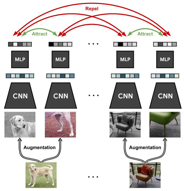
II: Self-supervised learning
Given a bunch of unlabeled samples ,
want to find “good” features
(e.g. so that a linear classifier on works with few samples)
One common approach: contrastive learning
![]()
![]()
Variants:
CPC, SimCLR, MoCo, SwAV, …
Mutual information isn't why SSL works!
InfoNCE approximates MI between "positive" views
But MI is invariant to transformations important to SSL!
![]()
Hilbert-Schmidt Independence Criterion (HSIC)
With a linear kernel:
Estimator based on kernel matrices:
- is the centering matrix
- is the kernel matrix on
- is the kernel matrix on
SSL-HSIC
(
is just an indicator of which source image it came from)
![]()
Target representation is output of
HSIC uses learned kernel
Your InfoNCE model is secretly a kernel method…
Very similar loss! Just different regularizer
When variance is small,
Clustering interpretation
SSL-HSIC estimates agreement of with cluster structure of
With linear kernels:
where is mean of the augmentations
Resembles BYOL loss with no target network (but still works!)
ImageNet results: linear evaluation
![]()
Transfer from ImageNet to classification tasks
![]()
III: Training implicit generative models
Given samples from a distribution over ,
we want a model that can produce new samples from
![]()
![]()
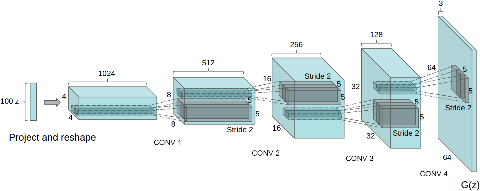
Generator networks
Fixed distribution of latents:
Maps through a network:
![]()
DCGAN generator [Radford+ ICLR-16]
How to choose ?
GANs and their flaws
- GANs [Goodfellow+ NeurIPS-14] minimize discriminator accuracy (like classifier test) between and
- Problem: if there's a perfect classifier, discontinuous loss, no gradient to improve it [Arjovsky/Bottou ICLR-17]
Disjoint at init:
:
![]()
:
![]()
- For usual , is supported on a countable union of manifolds with dim
- “Natural image manifold” usually considered low-dim
- Won't align at init, so won't ever align
WGANs and MMD GANs
- Integral probability metrics with “smooth” are continuous
- WGAN: a set of neural networks satisfying
- WGAN-GP: instead penalize near the data
- Both losses are MMD with
- Some kind of constraint on is important!
Non-smoothness of plain MMD GANs
Illustrative problem in , DiracGAN [Mescheder+ ICML-18]:
![]()
- Just need to stay away from tiny bandwidths
- …deep kernel analogue is hard.
- Instead, keep witness function from being too steep
- would give Wasserstein
- Nice distance, but hard to estimate
- Control on average, near the data
MMD-GAN with gradient control
- If gives uniformly Lipschitz critics, is smooth
- Original MMD-GAN paper [Li+ NeurIPS-17]: box constraint
- We [Bińkowski+ ICLR-18] used gradient penalty on critic instead
- Better in practice, but doesn't fix the Dirac problem…
New distance: Scaled MMD
Want to ensure
Can solve with …but too expensive!
Guaranteed if
Gives distance
Deriving the Scaled MMD
Smoothness of
![]()
Theorem: is continuous.
If has a density;
is Gaussian/linear/…;
is fully-connected, Leaky-ReLU, non-increasing width;
all weights in have bounded condition number;
then
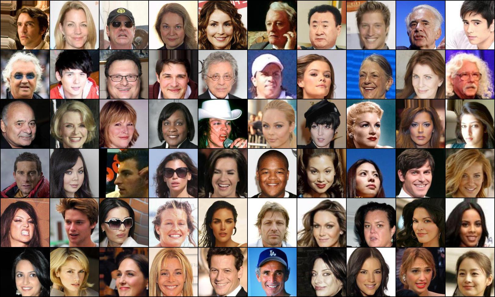
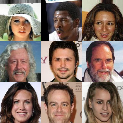
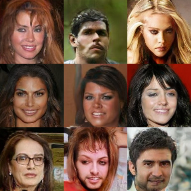
Results on CelebA
SN-SMMD-GAN
![]()
KID: 0.006
WGAN-GP
![]()
KID: 0.022
Evaluating generative models
![]()
Evaluating generative models
- Human evaluation: good at precision, bad at recall
- Likelihood: hard for GANs, maybe not right thing anyway
- Two-sample tests: always reject!
- Most common: Fréchet Inception Distance, FID
- Run pretrained featurizer on model and target
- Model each as Gaussian; compute
- Strong bias, small variance: very misleading
- Simple examples where
but
for reasonable sample size
- Our KID: instead. Unbiased, asymptotically normal
Training process on CelebA
IV: Unnormalized density/score estimation
- Problem: given samples with density
- Model is kernel exponential family: for any ,
i.e. any density with
- Gaussian : dense in all continuous distributions on compact domains
Density estimation with KEFs
- Fitting with maximum likelihood is tough:
- , are tough to compute
- Likelihood equations ill-posed for characteristic kernels
- We choose to fit the unnormalized model
- Could then estimate once after fitting if necessary
Unnormalized density / score estimation
- Don't necessarily need to compute afterwards
- , the “energy”, lets us:
- Find modes (global or local)
- Sample (with MCMC)
- …
- The score, , lets us:
- Run HMC for targets whose gradients we can't evaluate
- Construct Monte Carlo control functionals
- …
- Idea: minimize Fisher divergence
- Under mild assumptions,
- Can estimate with Monte Carlo
- Minimize regularized loss function:
- Representer theorem tells us minimizer of over is
![]()
![]()
Score matching in a subspace
- Best is in
- Find best
in dim subspace
in time
- : , time!
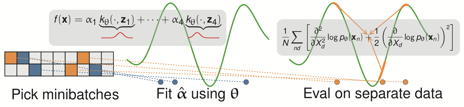
Meta-learning a kernel
- This was all with a fixed kernel and
- Good results need carefully tuned kernel and
- We can use a deep kernel as long as we split the data
- Otherwise it would always pick bandwidth 0
![]()
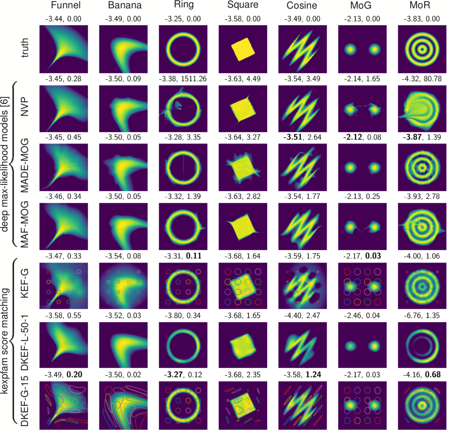
Results
- Learns local dataset geometry: better fits
- On real data: slightly worse likelihoods, maybe better “shapes” than deep likelihood models
Recap
Combining a deep architecture with a kernel machine that takes the higher-level learned representation as input can be quite powerful.
— Y. Bengio & Y. LeCun (2007), “Scaling Learning Algorithms towards AI”
- Two-sample testing [ICLR-17, ICML-20, NeurIPS-21]
- maximizing power criterion, for one task or many
- Self-supervised learning with HSIC [NeurIPS-21]
- Much better understanding of what's going on!
- Generative modeling with MMD GANs [ICLR-18, NeurIPS-18]
- Need a smooth loss function for the generator
- Score matching in exponential families [AISTATS-18, ICML-19]
- Avoid overfitting with closed-form fit on held-out data


 KID: 0.006
 KID: 0.022