Modern Kernel Methods
in Machine Learning:
Part II

Danica J. Sutherland(she/her)
Computer Science, University of British Columbia
ETICS "summer" school, Oct 2022

(Swipe or arrow keys to move through slides; for a menu to jump; to show more.)

Yesterday, we saw:

• RKHS is a function space,
• Reproducing property:
• Representer theorem:
• Can use to do kernel ridge regression, SVMs, etc

Today:

• Kernel mean embeddings of distributions
• Gaussian processes and probabilistic numerics
• Kernel approximations, for better computation
• Neural tangent kernels

Mean embeddings of distributions

• Represent point as :
• Represent distribution as :
  • Last step assumed e.g.
• Okay. Why?
  • One reason: ML on distributions [Szabó+ JMLR-16]
  • More common reason: comparing distributions

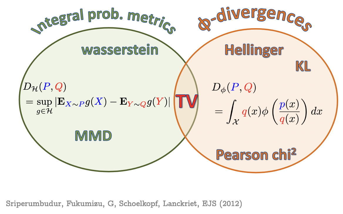
Maximum Mean Discrepancy

• Last line is Integral Probability Metric (IPM) form
• is called “witness function” or “critic”: high on , low on

MMD properties

• , symmetry, triangle inequality
• If is characteristic, then iff
  • i.e. is injective
  • Makes MMD a metric on probability distributions
  • Universal => characteristic
• Linear kernel: is just Euclidean distance between means

Application: Kernel Herding

• Want a "super-sample" from :
• If , error
• Greedily minimize the MMD:
• Get approximation instead of with random samples

Estimating MMD from samples

	1.0	0.2	0.6
	0.2	1.0	0.5
	0.6	0.5	1.0

	1.0	0.8	0.7
	0.8	1.0	0.6
	0.7	0.6	1.0

	0.3	0.1	0.2
	0.2	0.3	0.3
	0.2	0.1	0.4

MMD vs other distances

• MMD has easy estimator
  • block or incomplete estimators are for , but noisier
• For bounded kernel, estimation error
  • Independent of data dimension!
  • But, no free lunch…the value of the MMD generally shrinks with growing dimension, so constant error gets worse relatively

Application: Two-sample testing

• Given samples from two unknown distributions
• Question: is ?
• Hypothesis testing approach:
• Reject if

What's a hypothesis test again?

MMD-based testing

• : converges in distribution to…something
  • Infinite mixture of s, params depend on and
  • Can estimate threshold with permutation testing
• : asymptotically normal
• Any characteristic kernel gives consistent test…eventually
• Need enormous if kernel is bad for problem

Classifier two-sample tests

• is the accuracy of on the test set
• Under , classification impossible:
• With where ,
  get

Deep learning and deep kernels

• is one form of deep kernel
• Deep models are usually of the form
  • With a learned
• If we fix , have with
  • Same idea as NNGP approximation
• Generalize to a deep kernel:

Normal deep learning deep kernels

• Take
• Final function in will be
• With logistic loss: this is Platt scaling

“Normal deep learning deep kernels” – so?

• This definitely does not say that deep learning is (even approximately) a kernel method
• …despite what some people might want you to think
• We know theoretically deep learning can learn some things faster than any kernel method [see Malach+ ICML-21 + refs]
• But deep kernel learning ≠ traditional kernel models
  • exactly like how usual deep learning ≠ linear models

Optimizing power of MMD tests

• Asymptotics of give us immediately that , , are constants: first term usually dominates
• Pick to maximize an estimate of
• Use from before, get from U-statistic theory
• Can show uniform convergence of estimator
• Get better tests (even after data splitting)

Application: (S)MMD GANs

• An implicit generative model:
  • A generator net outputs samples from
  • Minimize estimate of on a minibatch
• MMD GAN:
• SMMD GAN:
  • Scaled MMD uses kernel properties to ensure smooth loss for by making witness function smooth [Arbel+ NeurIPS-18]
  • Uses
  • Standard WGAN-GP better thought of in kernel framework

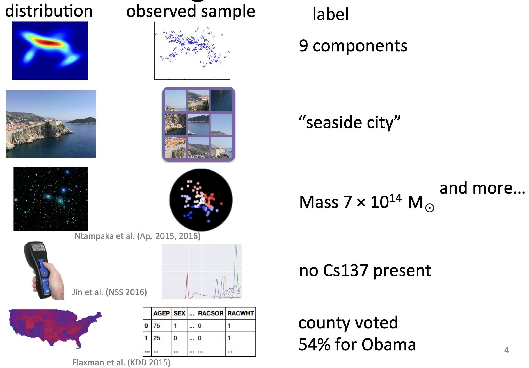
Application: distribution regression/classification/…

• We can define a kernel on distributions by, e.g.,
• Some pointers:
  [Muandet+ NeurIPS-12] [Sutherland 2016] [Szabó+ JMLR-16]

Example: age from face images [Law+ AISTATS-18]

Bayesian distribution regression: incorporate uncertainty

, , , ,

IMDb database [Rothe+ 2015]: 400k images of 20k celebrities

Independence

• iff for all measurable ,
• Let's implement for RKHS functions , :where is

Cross-covariance operator and independence

• If , then
• If ,
• If , are characteristic:
  • implies [Szabó/Sriperumbudur JMLR-18]
  • iff
  • iff (sum squared singular values)
    • HSIC: "Hilbert-Schmidt Independence Criterion"

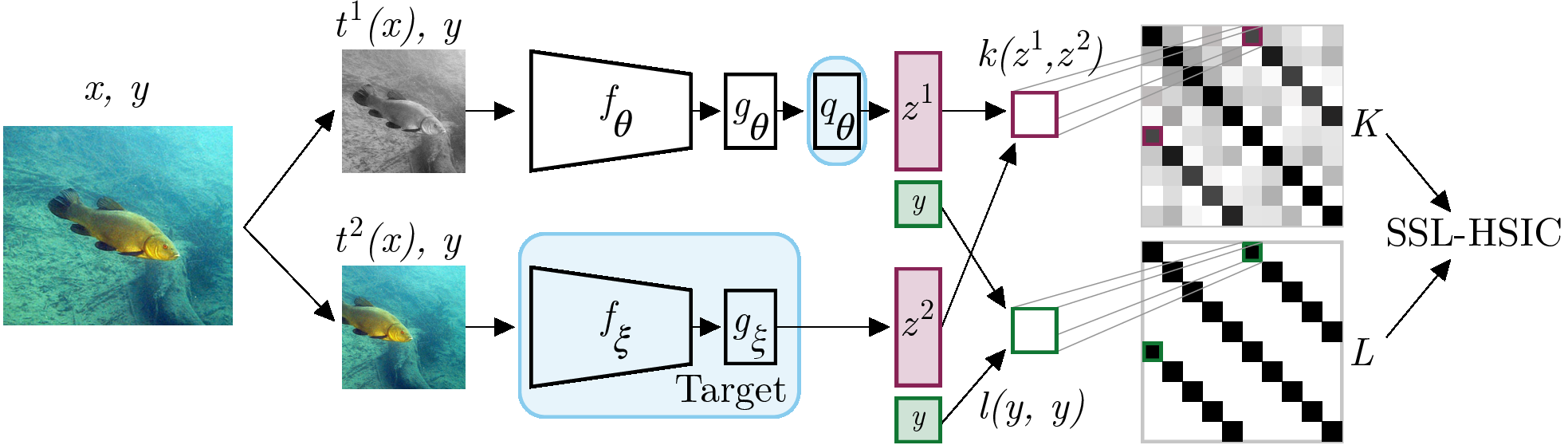
HSIC

• Linear case: is cross-covariance matrix,
  HSIC is squared Frobenius norm
• Default estimator (biased, but simple):
  where

HSIC applications

• Independence testing [Gretton+ NeurIPS-07]
• Clustering [Song+ ICML-07]
• Feature selection [Song+ JMLR-12]
• Self-supervised learning [Li+ NeurIPS-21]
• ⋮
• Broadly: easier-to-estimate, sometimes-nicer version of mutual information

Example: SSL-HSIC [Li+ NeurIPS-21]

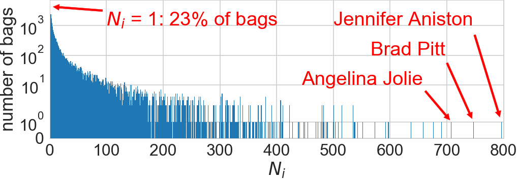
• Maximizes dependence between image features and its identity on a minibatch
• Using a learned deep kernel based on

Recap

• Mean embedding
• is 0 iff (for characteristic kernels)
• is 0 iff (for characteristic , )
• After break: last interactive session exploring testing
• More details:
  • Close connections to Gaussian processes [Kanagawa+ 'GPs and Kernel Methods' 2018]
  • Mean embeddings: survey [Muandet+ 'Kernel Mean Embedding of Distributions']